
Assignment 7
과제 7
| 과제 | 7 |
|---|---|
| 점수 | 0 |
| 제출 | False |
참조: \(\text{P6}\) in the exercise set 7.8 of the textbook
2차원 평면 상에서, 두 개의 점만 주어지면 우리는 두 점을 지나는 직선을 구할 수 있습니다. 예를들어, \((x_1,\,y_1)\) 와 \((x_2,\,y_2)\) 를 지나는 직선은,
\[\frac{y - y_1}{y_2 - y_1} - \frac{x - x_1}{x_2 - x_1} = 0\]인 것을 이미 알고 있습니다. 만약 세 개 이상의 점들이 주어진다면 어떨까요? 주어진 점들이 모두 한 직선안에 있다면, 점들을 모두 지나는 직선을 구해낼 수 있을 것입니다. 하지만, 어느 한 점이라도 일직선 상에서 벗어나있다면, 모든 점을 지나는 직선은 존재하지 않게 됩니다. 이럴 때, 주어진 점들을 ‘가장 잘’ 표현하는 직선(또는 특정 형태의 곡선)을 구하는 한 가지 방법으로 least square solution을 이용한 best approximation을 사용할 수 있습니다.
1. Linear model
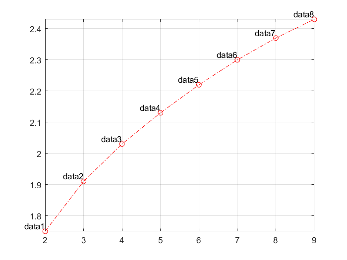
다음과 같은 데이터가 주어졌다고 하겠습니다:
| axis | data1 | data2 | data3 | data4 | data5 | data6 | data7 | data8 |
|---|---|---|---|---|---|---|---|---|
| \(\mathbf{x}\) | 2 | 3 | 4 | 5 | 6 | 7 | 8 | 9 |
| \(\mathbf{y}\) | 1.75 | 1.91 | 2.03 | 2.13 | 2.22 | 2.30 | 2.37 | 2.43 |
데이터들은 (거의 한 눈에 알 수 있듯이) 한 직선 위에 있지 않습니다. 우리는 주어진 데이터를 ‘가장 잘’ 표현하는 \(y = ax + b\)를 구하려 합니다.
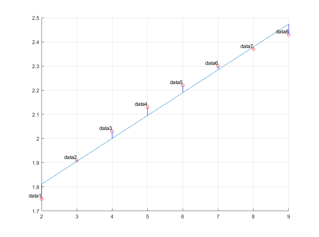
데이터 행렬 \(M\)를 구성하고,
\[M = \begin{bmatrix} 2 & 3 & 4 & 5 & 6 & 7 & 8 & 9\\ 1 & 1 & 1 & 1 & 1 & 1 & 1 & 1 \end{bmatrix}^T\]normal equation \(M^TM\mathbf{v} = M^T\mathbf{y}\), \(v = (a,\,b)\) 를 풀어서 직선을 구할 수 있습니다.
x = [2, 3, 4, 5, 6, 7, 8, 9]';
y = [1.75, 1.91, 2.03, 2.13, 2.22, 2.30, 2.37, 2.43]';

m = length(x);
t = linspace(min(x), max(x));
M = [x, ones(m,1)];
Y = y;                      % Set the least squares problem.
v = M \ Y;                  % Find the least squares solution.
a = v(1); b = v(2);         % Fitting constants a and b.
figure; hold on;
plot(x, y, 'ro');         % Plot given data points.
% Plot the fitting curve with a and b.
plot(t, a*t+b, 'color', [0 0.4470 0.7410]);
grid on;
title(sprintf('Linear model (y=%.3fx+%.3f)', a, b));
2. Exponential model
주어진 데이터
| axis | data1 | data2 | data3 | data4 | data5 | data6 | data7 | data8 |
|---|---|---|---|---|---|---|---|---|
| \(\mathbf{x}\) | 0 | 1 | 2 | 3 | 4 | 5 | 6 | 7 |
| \(\mathbf{y}\) | 3.9 | 5.3 | 7.2 | 9.6 | 12 | 17 | 23 | 31 |
를 가장 잘 표현하는 지수 모델 \(y = ae^{bx}\)를 구하려고 합니다. 등호의 양 쪽에 \(\log\)를 취하면,
\[Y = bx + A, \qquad Y :=\log{y}, \quad A := \log{a}\]를 얻을 수 있고,
\[\begin{align*} M &= \begin{bmatrix} 0 & 1 & 2 & 3 & 4 & 5 & 6 & 7\\ 1 & 1 & 1 & 1 & 1 & 1 & 1 & 1 \end{bmatrix}^T,\\ \mathbf{v} &= \begin{bmatrix} b & A \end{bmatrix}^T,\\ Y &= \begin{bmatrix} \log{3.9} & \log{5.3} & \log{7.2} & \log{9.6} & \log{12} & \log{17} & \log{23} & \log{31} \end{bmatrix}^T \end{align*}\]에 대하여 normal equation, \(M^TM\mathbf{v} = M^TY\), 을 풀어서 \(b\), \(a = e^A\)를 구할 수 있습니다.
x = [0, 1, 2, 3, 4, 5, 6, 7]';
y = [3.9, 5.3, 7.2, 9.6, 12, 17, 23, 31]';

m = length(x);
t = linspace(min(x), max(x));
M = [x, ones(m,1)]; Y = log(y); % Set the least squares problem.
v = M \ Y;                      % Find the least squares solution.
a = exp(v(2)); b = v(1);        % Fitting constants a and b.
figure; hold on;
plot(x, y, 'ro');                   % Plot given data points.
% Plot the fitting curve with a and b.
plot(t, a*exp(b*t), 'color', [0 0.4470 0.7410]);
grid on;
title(sprintf('Exponential model (y=%.3f*exp(%.3f*x))', a, b))
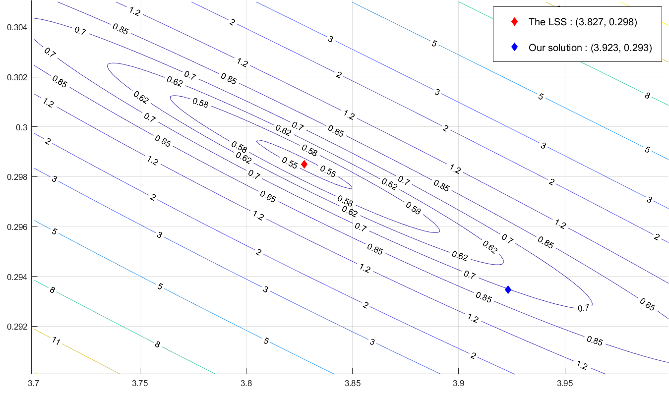
Linear model에서 normal equation을 풀어서 구한 solution은, 주어진 데이터와 linear model \(y = ax+b\)에 대한 least square solution(LSS) 입니다. 즉, 각 데이터의 \(y\)값들과의 거리의 제곱이 가장 작아지도록 하는 관점에서, linear model이 데이터를 ‘가장 잘’ 표현할 수 있도록 하는 \(a,\,b\)를 구한 것이죠.
하지만, exponential model 에서 구한 solution은 \(y = ae^{bx}\)가 아닌 \(Y = bx + A\)에 대한 LSS입니다. 다시 말하면, 각 데이터의 \(y\) 값들과의 거리가 아닌, \(\log{y}\)와의 거리가 가장 작아지도록 하는 solution을 구한 것입니다. 이 solution은 LSS와 같지 않습니다. 다음 그림은, \(E(a, b) := \sum_{i=1}^{8} (y_i - ae^{bx_i})^2\)를 최소화 하여 얻은 LSS와, 우리가 얻은 solution을 \(E\)의 level set들과 함께 표시한 것 입니다.
3. Logarithmic model
| axis | data1 | data2 | data3 | data4 | data5 | data6 | data7 | data8 |
|---|---|---|---|---|---|---|---|---|
| \(\mathbf{x}\) | 2 | 3 | 4 | 5 | 6 | 7 | 8 | 9 |
| \(\mathbf{y}\) | 4.07 | 5.30 | 6.21 | 6.79 | 7.32 | 7.91 | 8.23 | 8.51 |
이번에는, \(y = a + b\log(x)\) 모델을 이용하여 주어진 데이터를 피팅하겠습니다.
x = [2 3 4 5 6 7 8 9]';
y = [4.07 5.30 6.21 6.79 7.32 7.91 8.23 8.51]';

m = length(x);
t = linspace(min(x), max(x));
A = [ones(m,1) log(x)]; Y = y;	% Set the least squares problem.
v = A \ Y;                      % Find the least squares solution.
a = v(1); b = v(2);             % Fitting constants a and b.
figure; hold on;
plot(x, y, 'ro');               % Plot given data points.
% Plot the fitting curve with a and b.
plot(t, a + b*log(t), 'color', [0 0.4470 0.7410]);
grid on;
title(sprintf('Logarithmic model (y=%.3f+%.3f*ln(x))', a, b));
연습문제
앞선 1, 2, 3번의 모델들 중에서 원하는 모델을 선택하여 데이터 피팅을 할 수 있는 함수 LS_solver를 작성하세요. 주어진 데이터 x, y에 대하여,
>> LS_solver(x, y, 1);
은 Linear model을 이용한 데이터 피팅을,
>> LS_solver(x, y, 2);
은 Exponential model을 이용한 데이터 피팅을,
>> LS_solver(x, y, 3);
은 Logarithmic model을 이용한 데이터 피팅을 하도록 작성하세요.
Assignment 7
| Assignment | 7 |
|---|---|
| Score | 0 |
| Submission | False |
Reference: \(\text{P6}\) in the exercise set 7.8 of the textbook
On a 2D plane, given only two points, we can find a straight line through them. For example, the line through two points \((x_1,\,y_1)\) 와 \((x_2,\,y_2)\) is:
\[\frac{y - y_1}{y_2 - y_1} - \frac{x - x_1}{x_2 - x_1} = 0\]What if more than three points were given? If all of the given points are in a straight line, we will be able to find a straight line through all the points. However, if any point is out of a straight line, there will be no straight line passing through all the points. In this case, we can use the best approximation as one way to find the straight line (or curve of a specific shape) that represents ‘the best’ line for a given point.
1. Linear model
Let’s consider the following data:
| axis | data1 | data2 | data3 | data4 | data5 | data6 | data7 | data8 |
|---|---|---|---|---|---|---|---|---|
| \(\mathbf{x}\) | 2 | 3 | 4 | 5 | 6 | 7 | 8 | 9 |
| \(\mathbf{y}\) | 1.75 | 1.91 | 2.03 | 2.13 | 2.22 | 2.30 | 2.37 | 2.43 |
The data are not on a straight line (as we can almost see at a glance). We are trying to find \(y = ax + b\) which is ‘the best’ representative line of the given data.
Construct the data matrix \(M\),
\[M = \begin{bmatrix} 2 & 3 & 4 & 5 & 6 & 7 & 8 & 9\\ 1 & 1 & 1 & 1 & 1 & 1 & 1 & 1 \end{bmatrix}^T\]and we can find \(a\) and \(b\) by solving the normal equation \(M^TM\mathbf{v} = M^T\mathbf{y}\), \(v = (a,\,b)\).
x = [2, 3, 4, 5, 6, 7, 8, 9]';
y = [1.75, 1.91, 2.03, 2.13, 2.22, 2.30, 2.37, 2.43]';

m = length(x);
t = linspace(min(x), max(x));
M = [x, ones(m,1)];
Y = y;                      % Set the least squares problem.
v = M \ Y;                  % Find the least squares solution.
a = v(1); b = v(2);         % Fitting constants a and b.
figure; hold on;
plot(x, y, 'ro');         % Plot given data points.
% Plot the fitting curve with a and b.
plot(t, a*t+b, 'color', [0 0.4470 0.7410]);
grid on;
title(sprintf('Linear model (y=%.3fx+%.3f)', a, b));
2. Exponential model
For given data set:
| axis | data1 | data2 | data3 | data4 | data5 | data6 | data7 | data8 |
|---|---|---|---|---|---|---|---|---|
| \(\mathbf{x}\) | 0 | 1 | 2 | 3 | 4 | 5 | 6 | 7 |
| \(\mathbf{y}\) | 3.9 | 5.3 | 7.2 | 9.6 | 12 | 17 | 23 | 31 |
we are going to find a exponential model \(y = ae^{bx}\) which is the best fit of the data. Taking \(\log\) on both sides of the equality, we get
\[Y = bx + A, \qquad Y :=\log{y}, \quad A := \log{a},\]and let
\[\begin{align*} M &= \begin{bmatrix} 0 & 1 & 2 & 3 & 4 & 5 & 6 & 7\\ 1 & 1 & 1 & 1 & 1 & 1 & 1 & 1 \end{bmatrix}^T,\\ \mathbf{v} &= \begin{bmatrix} b & A \end{bmatrix}^T,\\ Y &= \begin{bmatrix} \log{3.9} & \log{5.3} & \log{7.2} & \log{9.6} & \log{12} & \log{17} & \log{23} & \log{31} \end{bmatrix}^T \end{align*}\]then by solving the normal equation, \(M^TM\mathbf{v} = M^TY\), we can get \(b\), \(a = e^A\).
x = [0, 1, 2, 3, 4, 5, 6, 7]';
y = [3.9, 5.3, 7.2, 9.6, 12, 17, 23, 31]';

m = length(x);
t = linspace(min(x), max(x));
M = [x, ones(m,1)]; Y = log(y); % Set the least squares problem.
v = M \ Y;                      % Find the least squares solution.
a = exp(v(2)); b = v(1);        % Fitting constants a and b.
figure; hold on;
plot(x, y, 'ro');                   % Plot given data points.
% Plot the fitting curve with a and b.
plot(t, a*exp(b*t), 'color', [0 0.4470 0.7410]);
grid on;
title(sprintf('Exponential model (y=%.3f*exp(%.3f*x))', a, b))
The solution obtained by solving the normal equation in Linear model is the least square solution(LSS) for the given data and linear model \(y = ax+b\). In other words, from the viewpoint of making the square of the distance between the \(y\) values of each data become the smallest, we found \(a,\,b\) that is ‘the best’ linear model to represent the data.
but, the solution obtained from exponential model is the LSS for \(Y = bx + A\), not \(y = ae^{bx}\). In other words, the solution was found so that the distance from \(\log{y}\) is the smallest, not the distance from the \(y\) values of each data. This solution is not the same as LSS. The following figure shows the LSS obtained by minimizing \(E(a, b) := \sum_{i=1}^{8} (y_i-ae^{bx_i})^2\) and the solution we obtained. It is displayed with the level sets of \(E\).
3. Logarithmic model
| axis | data1 | data2 | data3 | data4 | data5 | data6 | data7 | data8 |
|---|---|---|---|---|---|---|---|---|
| \(\mathbf{x}\) | 2 | 3 | 4 | 5 | 6 | 7 | 8 | 9 |
| \(\mathbf{y}\) | 4.07 | 5.30 | 6.21 | 6.79 | 7.32 | 7.91 | 8.23 | 8.51 |
This time, we will fit the given data using the model \(y = a + b\log(x)\).
x = [2 3 4 5 6 7 8 9]';
y = [4.07 5.30 6.21 6.79 7.32 7.91 8.23 8.51]';

m = length(x);
t = linspace(min(x), max(x));
A = [ones(m,1) log(x)]; Y = y;	% Set the least squares problem.
v = A \ Y;                      % Find the least squares solution.
a = v(1); b = v(2);             % Fitting constants a and b.
figure; hold on;
plot(x, y, 'ro');               % Plot given data points.
% Plot the fitting curve with a and b.
plot(t, a + b*log(t), 'color', [0 0.4470 0.7410]);
grid on;
title(sprintf('Logarithmic model (y=%.3f+%.3f*ln(x))', a, b));
Exercise
Write a function LS_solver that can fit data by selecting the desired model from the previous models 1, 2, and 3. Write code that will work for given data x, y if we enter
>> LS_solver(x, y, 1);
than it uses the linear model,
>> LS_solver(x, y, 2);
than it uses the exponential model and
>> LS_solver(x, y, 3);
than it uses a logarithmic model.
Leave a comment