Assignment 7

November 12, 2021 14 minute read

과제 7

0. 과제 6 추가 문제 해답

과제 4의 연습문제에서, 우리는 3가지 기본행연산 중 ‘두 행의 교환’을 사용하지 않고 가우스-조르단 소거법을 적용할 수 있는 행렬들에 대해서만 작동하는 rref 함수를 작성하였습니다. 여기서는 임의의 행렬에 대해 적용할 수 있는 my_rref.m함수를 작성하려 합니다. 아래에 주어진 가이드 코드의 빈칸을 채워서 코드를 완성하세요.

function rref_A = my_rref (A)
% Find the reduced row echelon form of A
% by performing Gauss - Jordan elimination with partial pivoting .
[m, n] = size (A);
rref_A = A; % Initialization of rref_A as A.

% Forward Phase with row interchanges .
rowIdx = 1; % Count row.
for colIdx = 1 : n
    % Find element to interchange two rows .
    [ maxEntry , maxIdx ] = max(abs( rref_A ( rowIdx :m, colIdx )));
    
    if maxEntry >= 1E-10 % If This column is a non - zero vector ,
        % Store index of pivot column .
        pivotCols( rowIdx ) = colIdx ;
        % Interchanging two rows .
        rref_A ([ rowIdx , maxIdx + rowIdx - 1], :) = rref_A ([ maxIdx + rowIdx - 1, rowIdx ], :);
        % Normalizing current row.
        rref_A ( rowIdx , :) = rref_A ( rowIdx , :) / rref_A ( rowIdx , colIdx );
        % Successive row operation .
        for r = rowIdx + 1 : m
            rref_A (r, :) = rref_A (r, :) - rref_A (r, colIdx ) * rref_A ( rowIdx , :);
        end
        rowIdx = rowIdx + 1; % Move onto the next row.
    end
    if rowIdx > m % If it was finished , stop .
        break
    end
end

% Backward phase.
preLding1Row = 0;
for pc = pivotCols (end:-1:1) % Find only the pivot columns .
    % This is looking for the index of row in which leading 1 is apeared .
    for lding1Row = m - preLding1Row : -1 : 1
        preLding1Row = preLding1Row + 1;
        if rref_A ( lding1Row , pc) >= 1E-10
            break
        end
    end
    for r = ( lding1Row - 1): -1 : 1
        % Add 'minus (r, pivotCol )-entry times the ith row ' to the kth row.
        rref_A (r, :) = rref_A (r, :) - rref_A (r, pc) * rref_A ( lding1Row , :);
    end
end
end

과제	7
점수	15
기한	Nov 18, 11:59 PM
다운로드	링크
제출 형식	순서쌍 (\(a\), \(b\))
제출 장소	KLMS assignment 7

참조: \(\text{P6}\) in the exercise set 7.8 of the textbook

2차원 평면 상에서, 두 개의 점만 주어지면 우리는 두 점을 지나는 직선을 구할 수 있습니다. 예를들어, 서로 다른 두 점 \((x_1,\,y_1)\) 와 \((x_2,\,y_2)\) 를 지나는 직선은,

\[\frac{y - y_1}{y_2 - y_1} - \frac{x - x_1}{x_2 - x_1} = 0\]

인 것을 이미 알고 있습니다. 만약 세 개 이상의 점들이 주어진다면 어떨까요? 주어진 점들이 모두 한 직선안에 있다면, 점들을 모두 지나는 직선을 구해낼 수 있을 것입니다. 하지만, 어느 한 점이라도 일직선 상에서 벗어나있다면, 모든 점을 지나는 직선은 존재하지 않게 됩니다. 이럴 때, 주어진 점들을 ‘가장 잘’ 표현하는 직선(또는 특정 형태의 곡선)을 구하는 한 가지 방법으로 least square solution을 이용한 best approximation을 사용할 수 있습니다.

1. Linear model

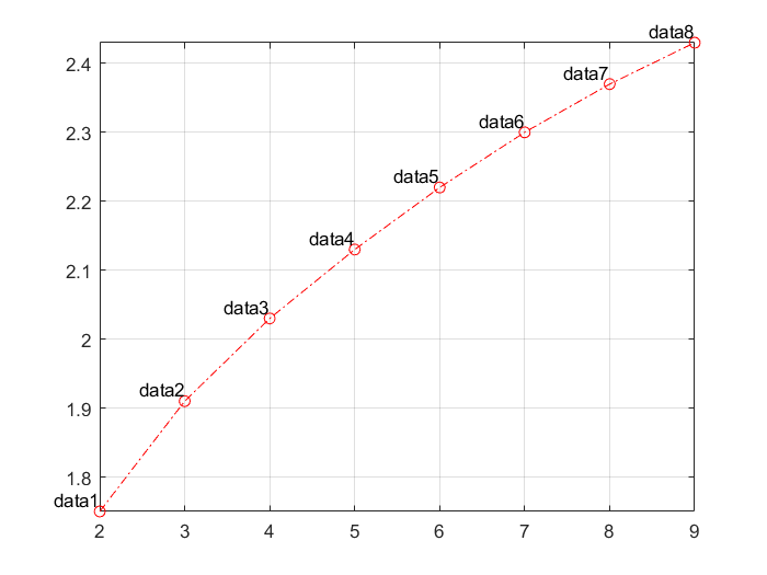
다음과 같은 데이터가 주어졌다고 하겠습니다:

axis	data1	data2	data3	data4	data5	data6	data7	data8
\(\mathbf{x}\)	2	3	4	5	6	7	8	9
\(\mathbf{y}\)	1.75	1.91	2.03	2.13	2.22	2.30	2.37	2.43

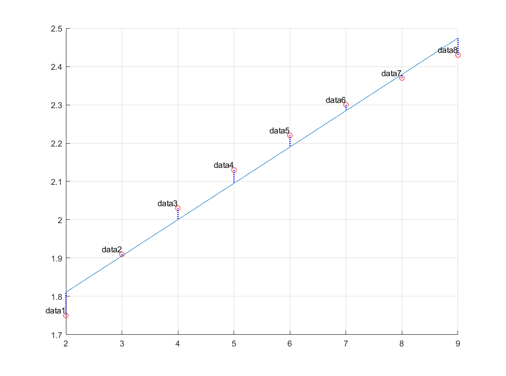
데이터들은 (한 눈에 알 수 있듯이) 한 직선 위에 있지 않기때문에, 모든 데이터를 다 지나가는 직선은 존재하지 않죠. 대신, 우리는 주어진 데이터를 ‘가장 잘’ 표현하는 \(y = ax + b\)를 구하려 합니다.

데이터 행렬 \(M\)를 구성하고,

\[M = \begin{bmatrix} 2 & 3 & 4 & 5 & 6 & 7 & 8 & 9\\ 1 & 1 & 1 & 1 & 1 & 1 & 1 & 1 \end{bmatrix}^T\]

normal equation \(M^TM\mathbf{v} = M^T\mathbf{y}\), \(v = (a,\,b)\) 를 풀어서 직선을 구할 수 있습니다.

x = [2, 3, 4, 5, 6, 7, 8, 9]';
y = [1.75, 1.91, 2.03, 2.13, 2.22, 2.30, 2.37, 2.43]';

m = length(x);
t = linspace(min(x), max(x));
M = [x, ones(m,1)]; 
Y = y;                      % Set the least squares problem.
v = M \ Y;                  % Find the least squares solution.
a = v(1); b = v(2);         % Fitting constants a and b.
figure; hold on;
plot(x, y, 'ro');         % Plot given data points.    
% Plot the fitting curve with a and b.
plot(t, a*t+b, 'color', [0 0.4470 0.7410]);
grid on;
title(sprintf('Linear model (y=%.3fx+%.3f)', a, b));

2. Exponential model

주어진 데이터

axis	data1	data2	data3	data4	data5	data6	data7	data8
\(\mathbf{x}\)	0	1	2	3	4	5	6	7
\(\mathbf{y}\)	3.9	5.3	7.2	9.6	12	17	23	31

를 가장 잘 표현하는 지수 모델 \(y = ae^{bx}\)를 구하려고 합니다. 등호의 양 쪽에 \(\log\)를 취하면,

\[Y = bx + A, \qquad Y :=\log{y}, \quad A := \log{a}\]

를 얻을 수 있고,

\[\begin{align*} M &= \begin{bmatrix} 0 & 1 & 2 & 3 & 4 & 5 & 6 & 7\\ 1 & 1 & 1 & 1 & 1 & 1 & 1 & 1 \end{bmatrix}^T,\\ \mathbf{v} &= \begin{bmatrix} b & A \end{bmatrix}^T,\\ Y &= \begin{bmatrix} \log{3.9} & \log{5.3} & \log{7.2} & \log{9.6} & \log{12} & \log{17} & \log{23} & \log{31} \end{bmatrix}^T \end{align*}\]

에 대하여 normal equation, \(M^TM\mathbf{v} = M^TY\), 을 풀어서 \(b\), \(a = e^A\)를 구할 수 있습니다.

x = [0, 1, 2, 3, 4, 5, 6, 7]';
y = [3.9, 5.3, 7.2, 9.6, 12, 17, 23, 31]';

m = length(x);
t = linspace(min(x), max(x));
M = [x, ones(m,1)]; Y = log(y); % Set the least squares problem.
v = M \ Y;                      % Find the least squares solution.
a = exp(v(2)); b = v(1);        % Fitting constants a and b.
figure; hold on;
plot(x, y, 'ro');                   % Plot given data points.    
% Plot the fitting curve with a and b.
plot(t, a*exp(b*t), 'color', [0 0.4470 0.7410]);
grid on;
title(sprintf('Exponential model (y=%.3f*exp(%.3f*x))', a, b))

Linear model에서 normal equation을 풀어서 구한 solution은, 주어진 데이터와 linear model \(y = ax+b\)에 대한 least square solution(LSS) 입니다. 즉, 각 데이터의 \(y\)값들과의 거리의 제곱이 가장 작아지도록 하는 관점에서, linear model이 데이터를 ‘가장 잘’ 표현할 수 있도록 하는 \(a,\,b\)를 구한 것이죠.

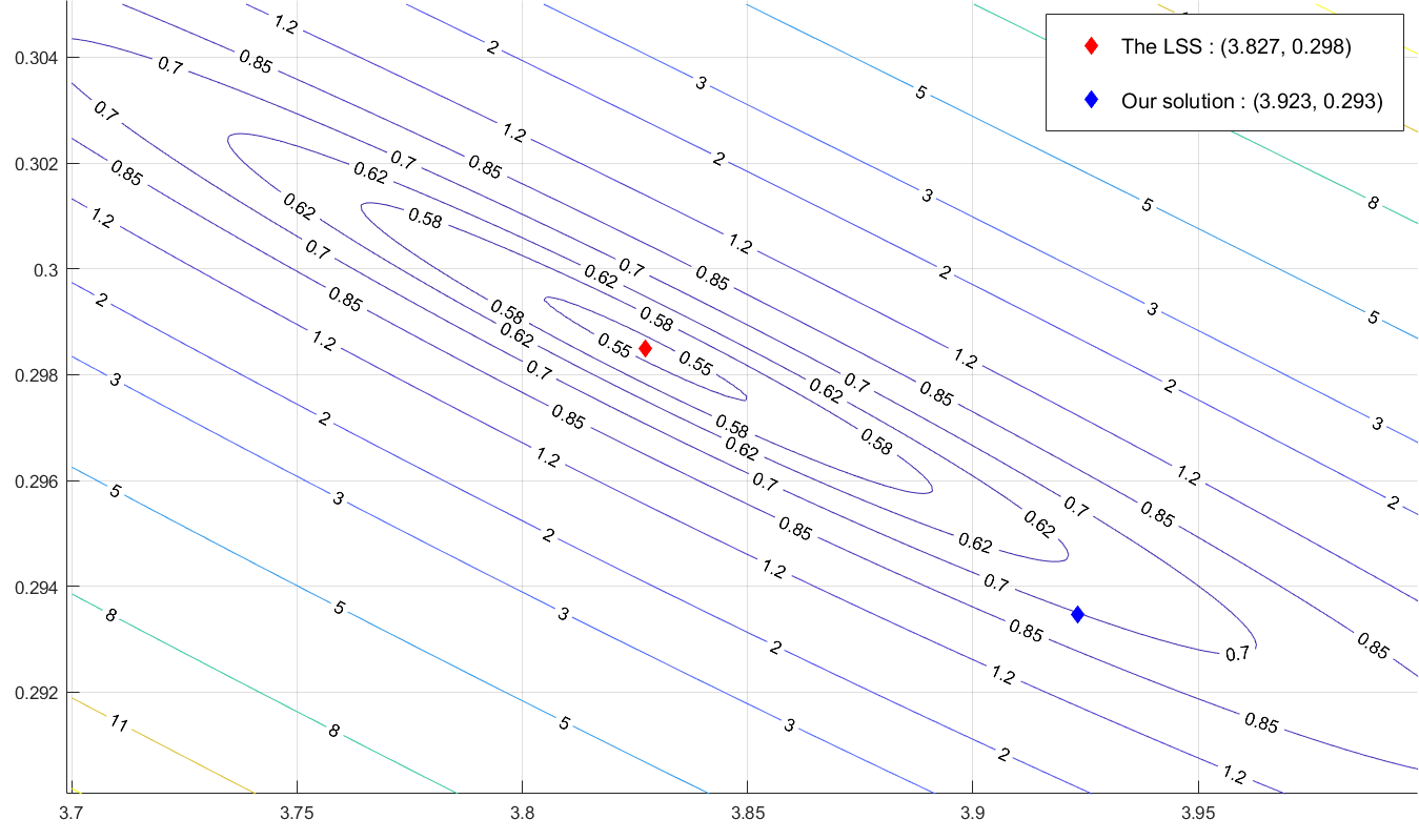
하지만, exponential model 에서 구한 solution은 \(y = ae^{bx}\)가 아닌 \(Y = bx + A\)에 대한 LSS입니다. 다시 말하면, 각 데이터의 \(y\) 값들과의 거리가 아닌, \(\log{y}\)와의 거리가 가장 작아지도록 하는 \(b\)와 \(A=\log{a}\)을 구한 것입니다. 주의해야 할 점은, 이 solution은 LSS와 같지 않다는 것입니다. 다음 그림은, \(E(a, b) := \sum_{i=1}^{8} (y_i - ae^{bx_i})^2\)를 최소화 하여 얻은 solution과 (즉 LSS), 우리가 얻은 solution (\(b,\,a\))을 \(E\)의 level set들과 함께 표시한 것 입니다. 비록 큰 차이가 나지는 않지만, 실제 LSS와는 분명한 차이가 있다는 걸 알 수 있습니다.

3. Logarithmic model

axis	data1	data2	data3	data4	data5	data6	data7	data8
\(\mathbf{x}\)	2	3	4	5	6	7	8	9
\(\mathbf{y}\)	4.07	5.30	6.21	6.79	7.32	7.91	8.23	8.51

이번에는, \(y = a + b\log(x)\) 모델을 이용하여 주어진 데이터를 피팅하겠습니다.

x = [2 3 4 5 6 7 8 9]';
y = [4.07 5.30 6.21 6.79 7.32 7.91 8.23 8.51]';

m = length(x);
t = linspace(min(x), max(x));
A = [ones(m,1) log(x)]; Y = y;	% Set the least squares problem.
v = A \ Y;                      % Find the least squares solution.
a = v(1); b = v(2);             % Fitting constants a and b.
figure; hold on;
plot(x, y, 'ro');               % Plot given data points.
% Plot the fitting curve with a and b.
plot(t, a + b*log(t), 'color', [0 0.4470 0.7410]);
grid on;
title(sprintf('Logarithmic model (y=%.3f+%.3f*ln(x))', a, b));

연습문제

앞선 1, 2, 3번의 모델들 중에서 원하는 모델을 선택하여 데이터 피팅을 할 수 있는 함수 LS_solver를 작성하세요. 주어진 데이터 x, y에 대하여,
```
 >> LS_solver(x, y, 1);
```
은 Linear model을 이용한 데이터 피팅을,
```
 >> LS_solver(x, y, 2);
```
은 Exponential model을 이용한 데이터 피팅을,
```
 >> LS_solver(x, y, 3);
```
은 Logarithmic model을 이용한 데이터 피팅을 하도록 작성하세요.
MAS109_assign7.p 파일을 다운받은 뒤 본인의 학번을 입력값으로 실행하세요. 이때 MAS109_assign7는 총 두개의 출력을 생성합니다, 두개의 출력들을 변수로 저장하세요. 두 개의 출력값들은, 순서대로 \(xy-\)좌표계에 주어진 데이터셋의 \(x\), \(y\) 좌표값들을 담고 있습니다. 즉, 첫번째 출력값은 \(x\)좌표를, 두번째 출력값은 \(y\)좌표를 의미합니다. 다음과 같은 함수 모델을 가정할 때:
\[y = axe^{bx}\]
주어진 데이터를 잘 표현하는 \(a\) 와 \(b\)를 구하세요.

제출 및 채점기준

연습문제 2번을 잘 읽고, 본인의 학번에 주어진 데이터를 잘 표현하기 위한 \(a\)와 \(b\)를 구하세요. 이 때, 반드시 normal equation을 구성하여서 문제를 해결하세요, 과목의 범위를 넘어서는 방법으로 구한 결과는 감점될 수 있습니다. 순서쌍 \((a,\,b)\)를 KLMS의 제출장소에 제출하세요.

Assignment 7

0. Solution for exercise problem in assignment 6

In the exercises of previous assignment 4, we wrote a function file that works only for matrices that can apply the Gauss-Jordan elimination without using the third elementary row operation, the ‘row exchange’. Here, we are going to write a MATLAB function my_rref.m that can be applied to an arbitrary matrix. Complete the code by filling in the blanks in the guide code given below.

function rref_A = my_rref (A)
% Find the reduced row echelon form of A
% by performing Gauss - Jordan elimination with partial pivoting .
[m, n] = size (A);
rref_A = A; % Initialization of rref_A as A.

% Forward Phase with row interchanges .
rowIdx = 1; % Count row.
for colIdx = 1 : n
    % Find element to interchange two rows .
    [ maxEntry , maxIdx ] = max(abs( rref_A ( rowIdx :m, colIdx )));
    
    if maxEntry >= 1E-10 % If This column is a non - zero vector ,
        % Store index of pivot column .
        pivotCols( rowIdx ) = colIdx ;
        % Interchanging two rows .
        rref_A ([ rowIdx , maxIdx + rowIdx - 1], :) = rref_A ([ maxIdx + rowIdx - 1, rowIdx ], :);
        % Normalizing current row.
        rref_A ( rowIdx , :) = rref_A ( rowIdx , :) / rref_A ( rowIdx , colIdx );
        % Successive row operation .
        for r = rowIdx + 1 : m
            rref_A (r, :) = rref_A (r, :) - rref_A (r, colIdx ) * rref_A ( rowIdx , :);
        end
        rowIdx = rowIdx + 1; % Move onto the next row.
    end
    if rowIdx > m % If it was finished , stop .
        break
    end
end

% Backward phase.
preLding1Row = 0;
for pc = pivotCols (end:-1:1) % Find only the pivot columns .
    % This is looking for the index of row in which leading 1 is appeared .
    for lding1Row = m - preLding1Row : -1 : 1
        preLding1Row = preLding1Row + 1;
        if rref_A ( lding1Row , pc) >= 1E-10
            break
        end
    end
    for r = ( lding1Row - 1): -1 : 1
        % Add 'minus (r, pivotCol )-entry times the ith row ' to the kth row.
        rref_A (r, :) = rref_A (r, :) - rref_A (r, pc) * rref_A ( lding1Row , :);
    end
end
end

Assignment	7
Score	15
Due date	Nov 18, 11:59 PM
Download	link
Submission format	an ordered pair (\(a\), \(b\))
Where to submit	KLMS assignment 7

Reference: \(\text{P6}\) in the exercise set 7.8 of the textbook

On a 2D plane, given only two points, we can find a straight line through them. For example, the line through two points \((x_1,\,y_1)\) 와 \((x_2,\,y_2)\) is:

\[\frac{y - y_1}{y_2 - y_1} - \frac{x - x_1}{x_2 - x_1} = 0\]

What if more than three points were given? If all of the given points are in a straight line, we will be able to find a straight line through all the points. However, if any point is out of a straight line, there will be no straight line passing through all the points. In this case, we can use the best approximation as one way to find the straight line (or curve of a specific shape) that represents ‘the best’ line for a given point.

1. Linear model

Let’s consider the following data:

axis	data1	data2	data3	data4	data5	data6	data7	data8
\(\mathbf{x}\)	2	3	4	5	6	7	8	9
\(\mathbf{y}\)	1.75	1.91	2.03	2.13	2.22	2.30	2.37	2.43

The data are not on a straight line (as we can almost see at a glance). We are trying to find \(y = ax + b\) which is ‘the best’ representative line of the given data.

Construct the data matrix \(M\),

\[M = \begin{bmatrix} 2 & 3 & 4 & 5 & 6 & 7 & 8 & 9\\ 1 & 1 & 1 & 1 & 1 & 1 & 1 & 1 \end{bmatrix}^T\]

and we can find \(a\) and \(b\) by solving the normal equation \(M^TM\mathbf{v} = M^T\mathbf{y}\), \(v = (a,\,b)\).

x = [2, 3, 4, 5, 6, 7, 8, 9]';
y = [1.75, 1.91, 2.03, 2.13, 2.22, 2.30, 2.37, 2.43]';

m = length(x);
t = linspace(min(x), max(x));
M = [x, ones(m,1)]; 
Y = y;                      % Set the least squares problem.
v = M \ Y;                  % Find the least squares solution.
a = v(1); b = v(2);         % Fitting constants a and b.
figure; hold on;
plot(x, y, 'ro');         % Plot given data points.    
% Plot the fitting curve with a and b.
plot(t, a*t+b, 'color', [0 0.4470 0.7410]);
grid on;
title(sprintf('Linear model (y=%.3fx+%.3f)', a, b));

2. Exponential model

For given data set:

axis	data1	data2	data3	data4	data5	data6	data7	data8
\(\mathbf{x}\)	0	1	2	3	4	5	6	7
\(\mathbf{y}\)	3.9	5.3	7.2	9.6	12	17	23	31

we are going to find a exponential model \(y = ae^{bx}\) which is the best fit of the data. Taking \(\log\) on both sides of the equality, we get

\[Y = bx + A, \qquad Y :=\log{y}, \quad A := \log{a},\]

and let

then by solving the normal equation, \(M^TM\mathbf{v} = M^TY\), we can get \(b\), \(a = e^A\).

x = [0, 1, 2, 3, 4, 5, 6, 7]';
y = [3.9, 5.3, 7.2, 9.6, 12, 17, 23, 31]';

m = length(x);
t = linspace(min(x), max(x));
M = [x, ones(m,1)]; Y = log(y); % Set the least squares problem.
v = M \ Y;                      % Find the least squares solution.
a = exp(v(2)); b = v(1);        % Fitting constants a and b.
figure; hold on;
plot(x, y, 'ro');                   % Plot given data points.    
% Plot the fitting curve with a and b.
plot(t, a*exp(b*t), 'color', [0 0.4470 0.7410]);
grid on;
title(sprintf('Exponential model (y=%.3f*exp(%.3f*x))', a, b))

The solution obtained by solving the normal equation in Linear model is the least square solution(LSS) for the given data and linear model \(y = ax+b\). In other words, from the viewpoint of making the square of the distance between the \(y\) values of each data become the smallest, we found \(a,\,b\) that is ‘the best’ linear model to represent the data.

but, the solution obtained from exponential model is the LSS for \(Y = bx + A\), not \(y = ae^{bx}\). In other words, the solution was found so that the distance from \(\log{y}\) is the smallest, not the distance from the \(y\) values of each data. This solution is not the same as LSS. The following figure shows the LSS obtained by minimizing \(E(a, b) := \sum_{i=1}^{8} (y_i-ae^{bx_i})^2\) and the solution we obtained. It is displayed with the level sets of \(E\).

3. Logarithmic model

axis	data1	data2	data3	data4	data5	data6	data7	data8
\(\mathbf{x}\)	2	3	4	5	6	7	8	9
\(\mathbf{y}\)	4.07	5.30	6.21	6.79	7.32	7.91	8.23	8.51

This time, we will fit the given data using the model \(y = a + b\log(x)\).

x = [2 3 4 5 6 7 8 9]';
y = [4.07 5.30 6.21 6.79 7.32 7.91 8.23 8.51]';

m = length(x);
t = linspace(min(x), max(x));
A = [ones(m,1) log(x)]; Y = y;	% Set the least squares problem.
v = A \ Y;                      % Find the least squares solution.
a = v(1); b = v(2);             % Fitting constants a and b.
figure; hold on;
plot(x, y, 'ro');               % Plot given data points.
% Plot the fitting curve with a and b.
plot(t, a + b*log(t), 'color', [0 0.4470 0.7410]);
grid on;
title(sprintf('Logarithmic model (y=%.3f+%.3f*ln(x))', a, b));

Exercise

Write a function LS_solver that can fit data by selecting the desired model from the previous models 1, 2, and 3. Write code that will work for given data x, y if we enter
```
 >> LS_solver(x, y, 1);
```
than it uses the linear model,
```
 >> LS_solver(x, y, 2);
```
than it uses the exponential model and
```
 >> LS_solver(x, y, 3);
```
than it uses a logarithmic model.
After downloading the MAS109_assign7.p file, run your student ID number as an input value. At this time, MAS109_assign7 will generate totally two outputs. Save the two outputs as distinct variables. The each output value contains the \(x\), \(y\) coordinate values of the given dataset in the \(xy-\) coordinate system in order. That is, the first output means \(x\) coordinates, and the second output means \(y\) coordinates. Assuming the following model:
\[y = axe^{bx},\]
Find \(a\) and \(b\) that approximate the given data well.

Submission and Scoring Criteria

Read exercise 2 carefully and find \(a\) and \(b\) to represent the data given in your student ID number. Be sure to solve the problem by composing a normal equation. You may lose points if the results is obtained in a way that is beyond the scope of this class. Submit the ordered pair \((a,\,b)\) to the KLMS.

Share on

Twitter Facebook

MATLAB TA

Assignment 7

과제 7

0. 과제 6 추가 문제 해답

1. Linear model

2. Exponential model

3. Logarithmic model

연습문제

제출 및 채점기준

Assignment 7

0. Solution for exercise problem in assignment 6

1. Linear model

2. Exponential model

3. Logarithmic model

Exercise

Submission and Scoring Criteria

Share on

Leave a comment