
Exercises 7.6 - 7.8
Chapter 7. Dimension and Structure
7.6 The Pivot Theorem and Its Implications
Exercise 7.7. (Finding a Basis with the Pivot Theorem)
Consider the vectors
\[\begin{align*} \mathbf{v}_{1} & =(1, \hspace{1mm} 2, \hspace{1mm} 4, \hspace{1mm} -6, \hspace{1mm} 11, \hspace{1mm} 23, \hspace{1mm} -14, \hspace{1mm} 0, \hspace{1mm} 2, \hspace{1mm} 2), \\ \mathbf{v}_{2} & = \hspace{1mm} (3, \hspace{1mm} 1, \hspace{1mm} -1, \hspace{1mm} 7, \hspace{1mm} 9, \hspace{1mm} 13, \hspace{1mm} -12, \hspace{1mm} 8, \hspace{1mm} 6, \hspace{1mm} -30), \\ \mathbf{v}_{3} & = \hspace{1mm} (5, \hspace{1mm} 5, \hspace{1mm} 7, \hspace{1mm} -5, \hspace{1mm} 31, \hspace{1mm} 59, \hspace{1mm} -40, \hspace{1mm} 8, \hspace{1mm} 10, \hspace{1mm}-26), \\ \mathbf{v}_{4} & = \hspace{1mm} (5, \hspace{1mm} 0, \hspace{1mm} -6, \hspace{1mm} 20, \hspace{1mm} 7, \hspace{1mm} 3, \hspace{1mm} -10, \hspace{1mm} 16, \hspace{1mm} 10, \hspace{1mm} -62). \end{align*}\]Use Algorithm \(1\) in Section \(7.6\) to find a subset of these vectors that forms a basis for span\(\{\mathbf{v}_{1}, \mathbf{v}_{2}, \mathbf{v}_{3}, \mathbf{v}_{4}\}\), and express those vectors not in the basis as linear combinations of basis vectors.
Solution.
v1 = [1 2 4 -6 11 23 -14 0 2 2]';
v2 = [3 1 -1 7 9 13 -12 8 6 -30]';
v3 = [5 5 7 -5 31 59 -40 8 10 -26]';
v4 = [5 0 -6 20 7 3 -10 16 10 -62]';

% Construct A whose column space is W=span(v1,v2,v3,v4).
A = [v1 v2 v3 v4];

% Find the reduced row echelon form R of A and the pivot columns of A.
[R, pivotcols] = rref(A);

format short;

disp('The pivot columns of the reduced row echelon form of A are');
disp(pivotcols);

% From the result, the leading 1's in R occur in columns 1 and 2.
% (i.e., the pivot columns of A are 1 and 2.)
% Hence, the basis vectors for W are v1 and v2.

disp('The reduced row echelon form R of A is'); disp(R);

% Furthermore, from the reduced row echelon form R of A,
% we can see that v3 = 2*v1 + v2, and v4 = -v1 + 2*v2.
MATLAB results.
The pivot columns of the reduced row echelon form of A are
     1     2

The reduced row echelon form R of A is
     1     0     2    -1
     0     1     1     2
     0     0     0     0
     0     0     0     0
     0     0     0     0
     0     0     0     0
     0     0     0     0
     0     0     0     0
     0     0     0     0
     0     0     0     0
Exercise 7.8. (Finding Bases for the Fundamental Spaces)
Consider the matrix
\[A = \left[\begin{array}{rrrr} 1 & \hspace{5mm} 3 & \hspace{5mm} 2 & \hspace{5mm} 1\\ -2 & -6 & 0 & -6 \\ 3 & 9 & 1 & 8 \\ -1 & -3 & -3 & -6 \\ 1 & 3 & 2 & 1 \\ 4 & 12 & 1 & 11 \end{array} \right].\]-
Use Algorithm 1 in Section 7.6 to find a subset of the column vectors of \(A\) that forms a basis for the column space of \(A\), and express each column vector of \(A\) that is not in that basis as a linear combination of the basis vectors.
-
Use Algorithm 2 in Section 7.6 to find a basis for the null space of the matrix \(A^{T}\).
Solution.
A = [1 3 2 1; -2 -6 0 -6; 3 9 1 8; -1 -3 -3 -6; 1 3 2 1; 4 12 1 11];

% Find the reduced row echelon form R of A and the pivot columns of A.
[R, pivotcols] = rref(A);

format short;

disp('The pivot columns of the reduced row echelon form of A are');
disp(pivotcols);
% From the result, the leading 1's in R occur in columns 1, 3, and 4.
% (i.e., the pivot columns of A are 1, 3, and 4.)
% Hence, the columns 1, 3, and 4 of A are a basis for the column space of A.

disp('The reduced row echelon form R of A is'); disp(R);
% Furthermore, from the reduced row echelon form R of A,
% we can see that v2 = 3*v1, where v1 = A(:, 1), and v2 = A(:, 2).
MATLAB results.
The pivot columns of the reduced row echelon form of A are
     1     3     4

The reduced row echelon form R of A is
     1     3     0     0
     0     0     1     0
     0     0     0     1
     0     0     0     0
     0     0     0     0
     0     0     0     0
7.7 The Projection Theorem and Its Implications
Exercise 7.9. (Standard Matrix for an Orthogonal Projection)
One way to find the standard matrix for the orthogonal projection onto a subspace \(W\) spanned by a set of vectors \(\{\mathbf{v}_{1}, \mathbf{v}_{2}, ..., \mathbf{v}_{k}\}\) is first to find a basis for \(W\), then create a matrix \(A\) that has the basis vectors as columns, and then use the Formula (27) in the Section 7.7.
-
Find the standard matrix for the orthogonal projection of \(\mathbb{R}^{4}\) onto the subspace \(W\) spanned by
\[\begin{align*} \mathbf{v}_{1} &= (1, \hspace{1mm} 2, \hspace{1mm} 3, \hspace{1mm} -4), &\mathbf{v}_{2} &= (2, \hspace{1mm}3, \hspace{1mm} -4, \hspace{1mm} 1), \\ \mathbf{v}_{3} &= (2, \hspace{1mm} -5, \hspace{1mm} 8, \hspace{1mm} -3), &\mathbf{v}_{4} &= (5, \hspace{1mm} 26, \hspace{1mm} -9, \hspace{1mm} -12), \\ \mathbf{v}_{5} &= (3, \hspace{1mm} -4, \hspace{1mm} 1, \hspace{1mm} 2). \end{align*}\] -
Use the matrix obtained in part 1. to find \(\mathrm{proj}_{W} \mathbf{x}\), where \(\mathbf{x} = (1, \hspace{1mm} 0, \hspace{1mm} -3, \hspace{1mm} 7)\).
-
Find \(\mathrm{proj}_{W^{\perp}} \mathbf{x}\) for the vector in part 2.
Solution.
v1 = [1 2 3 -4]'; v2 = [2 3 -4 1]'; v3 = [2 -5 8 -3]';
v4 = [5 26 -9 -12]'; v5 = [3 -4 1 2]';

% Set A that has v1,v2,v3,v4 and v5, as column vectors.
A = [v1 v2 v3 v4 v5];

% Find the reduced row echelon form R of A and the pivot columns of A.
[R, pivotcols] = rref(A);

% M is the matrix whose columns are a basis for the column space of A.
M = A(:, pivotcols);

% By (27) in section 7.7, find the standard matrix.
P = M * inv(M'* M) * M';

format short;
disp('The standard matrix for the orthogonal projection of R^4 onto W=col(A) is');
disp(P);

x = [1 0 -3 7]';
xproj = P*x;
xperp = x - xproj;
disp('The projection of x onto W=col(A) is'); disp(xproj');

disp('The projection of x onto the orthogonal complement of W=col(A) is');
disp(xperp');

% As a check, the dot product of the two projections should be zero.
disp('The dot product of the two projections is'); disp(dot(xproj, xperp));
MATLAB results.
The standard matrix for the orthogonal projection of R^4 onto W=col(A) is
    0.9992   -0.0144   -0.0161   -0.0195
   -0.0144    0.7551   -0.2737   -0.3314
   -0.0161   -0.2737    0.6941   -0.3703
   -0.0195   -0.3314   -0.3703    0.5517

The projection of x onto W=col(A) is
    0.9110   -1.5127   -4.6907    4.9534

The projection of x onto the orthogonal complement of W=col(A) is
    0.0890    1.5127    1.6907    2.0466

The dot product of the two projections is
  -5.3291e-15
7.8 Best Approximation and Least Squares
Exercise 7.10.
Make a function file LinearSolver.m to find a least squares solution of \(A\mathbf{x}=\mathbf{b}\) where \(A\) has full column rank. Complete the missing part referring to the comments. Using this function file, solve the linear system
and compare the output with the result of the MATLAB syntax A \ b.
Solution.
%--- This is a function file 'LinearSolver.m' ---%
function [rank_A, sol]=LinearSolver(A, b)
% We can skip the first output via `~`.
[~, n]=size(A);
rank_A=rank(A);

% Check that A has full column rank.
if rank_A<n
    fprintf('rank(A)=%d < %d  -> Not full column rank\n', rank_A, n);
    return; % If A does not have full column rank, then return.
else
    fprintf('rank(A)=%d = %d -> Full column rank\n', rank_A, n);
end

% From the reduced row echelon form of [A'*A |A'*b],
% find a solution to the normal equation A'Ax=A'b.

Aug=[A'*A A'*b];
rref_Aug=rref(Aug);
sol=rref_Aug(:,n+1);

fprintf('The least squares solution is');disp(sol');
end
You execute the followings:
A=[1 -1; 3 2; -2 4];
b=[4; 1; 3];
LinearSolver(A, b);
A\b
MATLAB results.
rank(A)=2 = 2 -> Full column rank
The least squares solution is    0.1789    0.5018

ans =

    0.1789
    0.5018
Exercise 7.11
The least squares method can be used to estimate the center \((h,\,k)\) of a circle \((x-h)^2+(y-k)^2=r^2\) using measured data points on its circumference. Suppose that the data points are
\[(x_1, y_1), (x_2, y_2), \cdots, (x_n, y_n)\]and rewrite the equation of the circle in the form
\[2xh+2yk+s=x^2+y^2 \tag{7.1}\]where
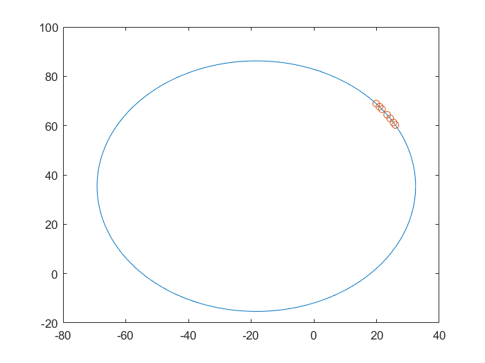
\[s=r^2-h^2-k^2 \tag{7.2}\]Substituting the data points in \((7.1)\) yields a linear system in the unknowns \(h\), \(k\), and \(s\), which can be solved by least squares to estimate their values. Equation \((7.2)\) can then be used to estimate \(r\). Use this method to approximate the center and radius of a circle from the measured data points on the circumference given in the accompanying table.
Table 7.1: Data points of Problem 7(b)
| axis | data1 | data2 | data3 | data4 | data5 | data6 | data7 |
|---|---|---|---|---|---|---|---|
| \(\mathbf{x}\) | 19.880 | 20.919 | 21.735 | 23.375 | 24.361 | 25.375 | 25.979 |
| \(\mathbf{y}\) | 68.874 | 67.676 | 66.692 | 64.385 | 62.908 | 61.292 | 60.277 |
Graph the circle you obtained and plot the data points with red circles in the same figure.
Solution. You execute the followings:
format short;

% given data
x = [19.880 20.919 21.735 23.375 24.361 25.375 25.979];
y = [68.874 67.676 66.692 64.385 62.908 61.292 60.277];

% number of data points.
[m, n]=size(x);

% construct the system matrix
A = [2*x' 2*y' ones(n,1)]; b = x.^2+y.^2;

% solve the normal equation
hks = inv(A'*A)*A'*b'
h = hks(1); k = hks(2); s = hks(3);

% compute the radius
r = sqrt(s+h^2+k^2);

figure;
theta = 0:0.01:2*pi;
xx = h+r*cos(theta);
yy = k+r*sin(theta);

% plot the obtained circle
plot(xx,yy);
hold on;

% plot the data points
plot(x, y, 'o');
MATLAB results.
hks =

  -18.3534
   35.4513
  986.5129
Leave a comment