Assignment 9

과제 9

과제	9
점수	0
제출	False
파일	다운로드

0. 연습문제 해답

0.1 과제 7 연습문제

1. 앞선 1, 2, 3번의 모델들 중에서 원하는 모델을 선택하여 데이터 피팅을 할 수 있는 함수 LS_solver를 작성하세요. 주어진 데이터 x, y에 대하여,

    >> LS_solver(x, y, 1);
   

   은 Linear model을 이용한 데이터 피팅을,

    >> LS_solver(x, y, 2);
   

   은 Exponential model을 이용한 데이터 피팅을,

    >> LS_solver(x, y, 3);
   

   은 Logarithmic model을 이용한 데이터 피팅을 하도록 작성하세요.

   Solution.

    function [a, b]=LS_solver(x, y, opt)
    % --------- function file LS_Solver --------- %
    % input data: x, y and opt
    %   if opt=1, linear model (y=a*x+b)
    %   if opt=2, exponential model (y=a*exp(b*x))
    %   if opt=3, logarithmic model (y=a+b*ln(x))
   
    [m1, n1]=size(x);   [m2, n2]=size(y);   % Sizes of the input datas.
    xx=linspace(min(x), max(x), 100);       % xx will be used to plot the fitting curve.
   
    if (m1~=1)||(m2~=1)||(n1~=n2)           % If the input data size is not proper,
        fprintf('Error: Improper input data.\n');   % print error message.
    elseif (opt==1)||(opt==2)||(opt==3)     % option = 1, 2, 3.
        figure; plot(x, y, 'o');            % Plot the given data points.
        hold on;                            % Ready to draw the next graph.
        if opt == 1                         % Linear model
            fprintf('Linear model\n');      % Print out the 'Linear model'.
            A=[x' ones(n1,1)]; Y=y';        % Set the least squares problem.
            sol=A\Y;                        % Find the least squares solution.
            a=sol(1); b=sol(2);             % Fitting constants a and b.
            plot(xx, a*xx+b);               % Plot the fitting curve with a and b.
            title('Linear model (y=a*x+b)');
        elseif opt == 2                   	% Exponential model
            fprintf('Exponential model\n'); % Print out the 'Exponential model'.
            A=[ones(n1,1) x']; Y=log(y');   % Set the least squares problem.
            sol=A\Y;                        % Find the least squares solution.
            a=exp(sol(1)); b=sol(2);        % Fitting constants a and b.
            plot(xx, a*exp(b*xx));          % Plot the fitting curve with a and b.
            title('Exponential model (y=a*exp(b*x))')
        elseif opt == 3              	    % Logarithmic model
            fprintf('Logarithmic model\n'); % Print out the 'Logarithmic model'.
            A=[ones(n1,1) log(x)']; Y=y';   % Set the least squares problem.
            sol=A\Y;                        % Find the least squares solution.
            a=sol(1); b=sol(2);             % Fitting constants a and b.
            plot(xx, a+b*log(xx));          % Plot the fitting curve with a and b.
            title('Logarithmic model (y=a+b*ln(x))');
        end
        hold off;                           % No more graph.
    else                                    % for invalid [opt]
        fprintf('Error: Improper option value.\n'); % error message.
        return                              % Return the process.
    end
    end
   

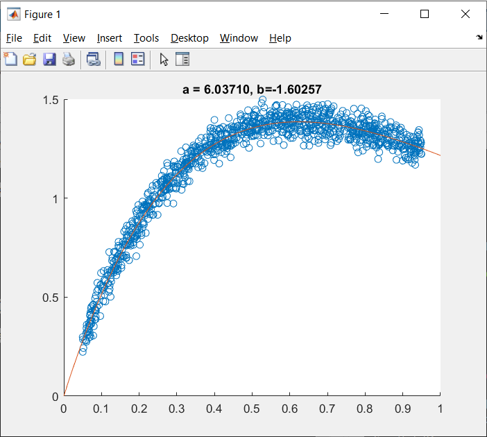
2. MAS109_assign7.p 파일을 다운받은 뒤 본인의 학번을 입력값으로 실행하세요. 이때 MAS109_assign7는 총 두개의 출력을 생성합니다, 두개의 출력들을 변수로 저장하세요. 두 개의 출력값들은, 순서대로 \(xy-\)좌표계에 주어진 데이터셋의 \(x\), \(y\) 좌표값들을 담고 있습니다. 즉, 첫번째 출력값은 \(x\)좌표를, 두번째 출력값은 \(y\)좌표를 의미합니다. 다음과 같은 함수 모델을 가정할 때:

   \[y = axe^{bx}\]

   주어진 데이터를 잘 표현하는 \(a\) 와 \(b\)를 구하세요.

   Solution. 학번이 20219999라고 가정하면,

    >> [x, y] = MAS109_assign7(20219999);
   

   을 입력하여서 x와 y를 얻을 수 있습니다. 주어진 함수 모델

   \[y = axe^{bx}\]

   의 양 변에 \(log\)를 취하면,

   \[log(y) = log(a) + log(x) + bx\quad \Rightarrow \quad log(y) - log(x) = log(a) + bx\]

   를 얻을 수 있고, 우항의 선형 모델의 계수들 \(log(a)\)와 \(b\)를 구하는 normal equation을 구성하여 문제를 해결할 수 있다.

    A = [ones(length(x), 1), x'];
    B = log(y)' - log(x)';
    C = A \ B;
   
    a = exp(C(1));
    b = C(2);
   
    xx = 0:0.01:1;
    yy = a .* xx .* exp(b.*xx);
   
    ab = sprintf('a = %.5f, b=%.5f', a, b);
   
    figure;
    scatter(x, y);
    hold on;
    plot(xx, yy);
    title(ab)
   

   MATLAB result.

   

0.2 과제 8 연습문제

1. MGS의 알고리즘을 참고하여, modified Gram-Schmidt를 수행하는 코드를 작성해보세요.

   Solution.

    %--- The following is the function file 'MGramSchmidt.m'. ---%
   
    % Find an orthonormal basis for col(A) when A has full column rank.
    function Q = MGramSchmidt(A)
   
    [m, n] = size(A);
   
    % Initialize the matrix Q as an m*n zero matrix.
    Q = zeros(m, n);
    for i = 1 : n
        % v begins as jth column of A.
        v = A(:, i);
        for j = 1 : i-1
            % Subtract each component of orthogonal projection of v
            % onto the subspace spanned by the vector Q(:, i).
            q = Q(:, j);
            v = v - (q' * v) * q;
        end
        Q(:, i) = v / norm(v); % Normalize v by its 2-norm.
    end
    end
    % Q is an m*n matrix whose columns form an orthonormal basis for col(A).
   

2. Classical GS와 modified GS를 비교하세요.

   임의 행렬

   1. 임의의 \(100 \times 100\) 행렬 \(A\)를 생성하세요. rank명령어를 사용하여 \(A\)가 non-singular인 것을 확인하세요.
      (높은 확률로 \(A\)는 non-singular matrix입니다, 만약 \(A\)가 singular matrix라면 다시 생성하세요.)

   2. \(\mbox{col}(A)\)의 orthonormal basis를 구성하세요. CGS를 이용한 결과를 \(Q_1\), MGS를 이용한 결과를 \(Q_2\)라고 할 때, 단위행렬과의 오차를 비교하세요.

   Solution.

    A = rand(100);
    fprintf('Rank of A : %d\n', rank(A));
   
    Q1 = CGramSchmidt(A);       % classical Gram-Schmidts
    Q2 = MGramSchmidt(A);       % modified Gram-Schmidts
   
    E1 = norm(Q1' * Q1 - eye(100));
    E2 = norm(Q2' * Q2 - eye(100));
    fprintf('Error of CGS = %g\n', E1)
    fprintf('Error of MGS = %g\n', E2)
   

   MATLAB results.

    Rank of A : 100
    Error of CGS = 2.96812e-12
    Error of MGS = 8.67502e-14
   

   상대적으로 좋은 행렬 \(A\)에 대해서는, CGS를 이용한 결과와 MGS를 이용한 결과가 크게 차이나지 않습니다.

   안 좋은 행렬 (Ill-conditioned matrix)

   1. 수치적으로 좋지않은 행렬 \(B\)를 생성하세요:

   2. CGS를 이용해 얻은 결과를 \(P_1\), MGS를 이용한 결과를 \(P_2\)라고 할 때, 단위행렬과의 오차를 비교하세요.

   Solution.

    B = 10^-5 * rand() * eye(100) + hilb(100);
   
    P1 = CGramSchmidt(B);
    P2 = MGramSchmidt(B);
   
    E1 = norm(P1' * P1 - eye(100));
    E2 = norm(P2' * P2 - eye(100));
    fprintf('Error of CGS = %g\n', E1)
    fprintf('Error of MGS = %g\n', E2)
   

   MATLAB results.

    Error of CGS = 87.6346
    Error of MGS = 3.7332e-11
   

   상대적으로 나쁜 행렬 \(B\)에 대해서는, CGS의 결과는 제대로된 orthogonal vector들을 구성하지 못합니다. 반면에, MGS는 괜찮은 결과들을 생성합니다.

---

MNIST dataset은 0 부터 9까지의 손글씨가 쓰여진 70000장의 이미지들로 이루어져 있습니다.

MNIST examples: https://en.wikipedia.org/wiki/MNIST_database

각 이미지는 \(28 \times 28\)의 크기를 가지며, 정답숫자와 함께 제공됩니다. 우리는 이 과제에서, best approximation을 이용한 MNIST의 손글씨 이미지 분류 작업을 해보려 합니다.

1. MNIST dataset 불러오기

문서에 첨부된 파일을 다운받은 후 압축을 해제하세요. 총 네개의 mat파일을 얻어야 합니다.

파일명	설명
train_image.mat	60000장의 손글씨 이미지들 입니다. train_image의 이미지들을 이용하여 best approximate solution을 구하려 합니다.
train_target.mat	train_image의 각 이미지에 대한 정답 숫자들을 순서대로 포함하고 있습니다.
test_image.mat	10000장의 손글씨 이미지들 입니다. train_image를 통해 얻어낸 solution을 검증하기 위해 사용합니다.
test_target.mat	test_image의 정답 숫자들 입니다.

매트랩에 다음 명령어들을 순서대로 입력하여 작업 공간에 데이터를 불러옵니다. 또한, 각 데이터의 형을 double로 지정합니다.

load('training_image.mat'); train_x = double(train_x);
load('training_target.mat'); train_y = double(train_y);
load('test_image.mat'); test_x = double(test_x);
load('test_target.mat'); test_y = double(test_y);

작업 공간에 4개의 변수가 생성되었는지 확인하세요.

Name          Size                      Bytes  Class  

test_x       28x28x10000             62720000  double              
test_y        1x10000                   80000  double              
train_x      28x28x60000            376320000  double              
train_y       1x60000                  480000  double  

2. Normal equation 구성 및 풀이 [0과 1 분류]

우선은 0과 1 단 두개의 숫자만 구분하도록 하는 solution을 구해보겠습니다. 정답 숫자가 0 또는 1인 데이터만 추출하여 변수를 재구성합니다.

% find indices whose value is either 0 or 1.
train_idx = [find(train_y == 0), find(train_y == 1)];
test_idx = [find(test_y == 0), find(test_y == 1)];

% Leave only data that are 0 or 1.
train_x = train_x(:, :, train_idx); train_y = train_y(:, train_idx);
test_x = test_x(:, :, test_idx);    test_y = test_y(:, test_idx);

각 행이 하나의 이미지로 이루어진 데이터 행렬 \(M\)을 구성하기 위해 train_x에 reshape명령어를 사용합니다.

M = reshape(train_x, 28^2, [])';    % [] means that 'matche dimension automatically'.
y = train_y';

(거의 자명하게도) \(Mx=y\)를 만족하는 \(y\)는 존재하지 않습니다. 따라서 우리는 best approximate solution을 구하려고 합니다.

1. 간단하게, 매트랩의 \ 구문을 사용하여 solution을 구할 수 있습니다. \는 자동으로 가장 적합한 solution을 구해줄 것 입니다.

    x = M \ y;  % the most simple way.
   

   하지만, 이 경우 \ 는 상당히 느리게 작동할 뿐 아니라, 우리 수준에서는 어떻게 solution을 구해주는지 이해하기 힘듭니다.

2. Normal equation을 직접 구성하여 solution을 구할 수도 있습니다. 이 때, linear system의 해를 구해주는 linsolve 명령어를 사용합니다.
   (이 경우, linsolve는 \(LDU\)-분해를 이용하여 해를 구합니다. 또한, \를 사용해도 역시 같은 알고리즘을 이용합니다.)

    A = M' * M;
    b = M' * y;
    x = linsolve(A, b);
   

   만약, 여러분이 위 코드를 그대로 사용하여 solution을 구했다면, 구해진 solution은 매우 잘못된 값을 포함하고 있을 확률이 높습니다. 이 것은 \(A\)의 원소가 대체적으로 0에 가까우며, 아주 적은량의 원소만 매우 크게 나타나서 수치적으로 불안정하기 때문입니다. 수치적 안정성을 높이는 방법은 여러가지가 있을 수 있지만, 여기서는 가장 간단하게 \(A\)에 작은 noise(perturbation)를 더하는 방법으로 해결하겠습니다. 물론, 이 방법으로 구해지는 solution은 실제값과는 조금 다릅니다. 하지만 여기서는 작은 오차는 무시하도록 합시다.
   (이 부분은 이해하지 않고 넘어가도 됩니다.)

    A = M' * M + rand(size(M, 2)) * 0.001;  % add random perturbation.
    b = M' * y;
    x = linsolve(A, b);
   

1과 2의 소요시간을 각각 확인해보죠.

%% method 1
tic; x = M \ y; toc;
%% method 2
tic;
A = M' * M + rand(size(M, 2)) * 0.001;
b = M' * y;
x = inv(A) * b; 
toc;

3. Solution 검증

앞서 불러온 0과 1로만 재구성 된 test데이터들을 이용하여 데이터 행렬 \(T\)와 \(z\)를 만듭니다.

T = reshape(test_x, 28^2, [])';
z = test_y';

앞서 구한 solution \(x\)를 이용하여 예측값 \(w\)를 구한 뒤, 반올림하여 \(z\)의 값과 비교합니다.

w = T * x;   % compute the prediction by the best approximate solution `x`
acc = sum(round(w) == z) / length(w);  % compute the accuracy: (# of correct answers) / (# of data points)
fprintf('Accuracy = %.2f %% \n', acc * 100)

우리가 만들어낸 모델(solution \(x\))은 98%가 넘는 정확도를 가지는, 꽤 정확한 분류모델인 걸 알 수 있습니다.

4. 더 많은 숫자 분류

이제 0과 1뿐만 아니라 더 많은 숫자들을 분류해 보겠습니다. 먼저 분류하고 싶은 숫자들을 지정한 뒤,

num_for_use = [0, 1, 2, 3];

for문을 활용하여 분류하고 싶은 숫자들만 골라내겠습니다. 구성 방식은 위와 완전히 같습니다.

train_idx = [];     % create empty idcies
test_idx = [];
for i = num_for_use
    train_idx = [train_idx, find(train_y == i)];
    test_idx = [test_idx, find(test_y == i)];
end

이제, 나머지 부분은 앞선 예제와 같습니다. 0, 1, 2, 3 네 개의 숫자를 분류하는 모델의 정확도는 70% 정도입니다.

연습문제

1. 여러개의 숫자를 분류하는 모델을 만들어보세요.

2. 위의 내용을 그대로 따라서 0과 9 두개의 숫자를 분류하는 모델을 만들고 검증 해보세요. 실제로는 0과 1을 분류하는 모델과 똑같이, 98% 정도의 정확도가 나와야 합니다. 여러분이 얻은 결과는 어떤가요?

   결과가 예상과 다르다면, 어느 부분에서 달라졌는지 생각해보고 수정해보세요.

---

Assignment 9

Assignment	9
Score	0
Submission	False
Files	Download

0. Solutions for previous assignments

0.1 Assignment 7

1. Write a function LS_solver that can fit data by selecting the desired model from the previous models 1, 2, and 3. Write code that will work for given data x, y if we enter

    >> LS_solver(x, y, 1);
   

   than it uses the linear model,

    >> LS_solver(x, y, 2);
   

   than it uses the exponential model and

    >> LS_solver(x, y, 3);
   

   than it uses a logarithmic model.

   Solution.

    function [a, b]=LS_solver(x, y, opt)
    % --------- function file LS_Solver --------- %
    % input data: x, y and opt
    %   if opt=1, linear model (y=a*x+b)
    %   if opt=2, exponential model (y=a*exp(b*x))
    %   if opt=3, logarithmic model (y=a+b*ln(x))
   
    [m1, n1]=size(x);   [m2, n2]=size(y);   % Sizes of the input datas.
    xx=linspace(min(x), max(x), 100);       % xx will be used to plot the fitting curve.
   
    if (m1~=1)||(m2~=1)||(n1~=n2)           % If the input data size is not proper,
        fprintf('Error: Improper input data.\n');   % print error message.
    elseif (opt==1)||(opt==2)||(opt==3)     % option = 1, 2, 3.
        figure; plot(x, y, 'o');            % Plot the given data points.
        hold on;                            % Ready to draw the next graph.
        if opt == 1                         % Linear model
            fprintf('Linear model\n');      % Print out the 'Linear model'.
            A=[x' ones(n1,1)]; Y=y';        % Set the least squares problem.
            sol=A\Y;                        % Find the least squares solution.
            a=sol(1); b=sol(2);             % Fitting constants a and b.
            plot(xx, a*xx+b);               % Plot the fitting curve with a and b.
            title('Linear model (y=a*x+b)');
        elseif opt == 2                   	% Exponential model
            fprintf('Exponential model\n'); % Print out the 'Exponential model'.
            A=[ones(n1,1) x']; Y=log(y');   % Set the least squares problem.
            sol=A\Y;                        % Find the least squares solution.
            a=exp(sol(1)); b=sol(2);        % Fitting constants a and b.
            plot(xx, a*exp(b*xx));          % Plot the fitting curve with a and b.
            title('Exponential model (y=a*exp(b*x))')
        elseif opt == 3              	    % Logarithmic model
            fprintf('Logarithmic model\n'); % Print out the 'Logarithmic model'.
            A=[ones(n1,1) log(x)']; Y=y';   % Set the least squares problem.
            sol=A\Y;                        % Find the least squares solution.
            a=sol(1); b=sol(2);             % Fitting constants a and b.
            plot(xx, a+b*log(xx));          % Plot the fitting curve with a and b.
            title('Logarithmic model (y=a+b*ln(x))');
        end
        hold off;                           % No more graph.
    else                                    % for invalid [opt]
        fprintf('Error: Improper option value.\n'); % error message.
        return                              % Return the process.
    end
    end
   

2. After downloading the MAS109_assign7.p file, run your student ID number as an input value. At this time, MAS109_assign7 will generate totally two outputs. Save the two outputs as distinct variables. The each output value ​​contains the \(x\), \(y\) coordinate values ​​of the given dataset in the \(xy-\) coordinate system in order. That is, the first output means \(x\) coordinates, and the second output means \(y\) coordinates. Assuming the following model:

   \[y = axe^{bx},\]

   Find \(a\) and \(b\) that approximate the given data well.

   Solution. For a student with ID number 20219999, one can get x and y by entering the following command:

    >> [x, y] = MAS109_assign7(20219999);
   

   For given functional model

   \[y = axe^{bx}\, ,\]

   we can get the following form by applying \(log\) to the both side of the equality,

   \[log(y) = log(a) + log(x) + bx\quad \Rightarrow \quad log(y) - log(x) = log(a) + bx\]

   and we can construct a normal equation for the linear model in the right hand side.

    A = [ones(length(x), 1), x'];
    B = log(y)' - log(x)';
    C = A \ B;
   
    a = exp(C(1));
    b = C(2);
   
    xx = 0:0.01:1;
    yy = a .* xx .* exp(b.*xx);
   
    ab = sprintf('a = %.5f, b=%.5f', a, b);
   
    figure;
    scatter(x, y);
    hold on;
    plot(xx, yy);
    title(ab)
   

   MATLAB result.

   

0.2 Assignment 8

1. Write a code that executes modified Gram-Schmidt by referring to the algorithm of MGS.

   Solution.

    %--- The following is the function file 'MGramSchmidt.m'. ---%
   
    % Find an orthonormal basis for col(A) when A has full column rank.
    function Q = MGramSchmidt(A)
   
    [m, n] = size(A);
   
    % Initialize the matrix Q as an m*n zero matrix.
    Q = zeros(m, n);
    for i = 1 : n
        % v begins as jth column of A.
        v = A(:, i);
        for j = 1 : i-1
            % Subtract each component of orthogonal projection of v
            % onto the subspace spanned by the vector Q(:, i).
            q = Q(:, j);
            v = v - (q' * v) * q;
        end
        Q(:, i) = v / norm(v); % Normalize v by its 2-norm.
    end
    end
    % Q is an m*n matrix whose columns form an orthonormal basis for col(A).
   

2. Compare Classical GS and Modified GS.

   Random matrix

   1. Generate a random \(100 \times 100\) matrix \(A\). Check that \(A\) is non-singular using the rank command.
      (There is a high probability that \(A\) is a non-singular matrix, if \(A\) is a singular matrix, recreate it.)

   2. Generate an orthonormal basis of \(\mbox{col}(A)\). Let the result using CGS be \(Q_1\) and the result using MGS be \(Q_2\). Compare the error with the unit matrix.

   Solution.

    A = rand(100);
    fprintf('Rank of A : %d\n', rank(A));
   
    Q1 = CGramSchmidt(A);       % classical Gram-Schmidts
    Q2 = MGramSchmidt(A);       % modified Gram-Schmidts
   
    E1 = norm(Q1' * Q1 - eye(100));
    E2 = norm(Q2' * Q2 - eye(100));
    fprintf('Error of CGS = %g\n', E1)
    fprintf('Error of MGS = %g\n', E2)
   

   MATLAB results.

    Rank of A : 100
    Error of CGS = 2.96812e-12
    Error of MGS = 8.67502e-14
   

   For the relatively good matrix \(A\), the results with CGS and MGS are nearly identical.

   Bad matrix (Ill-conditioned matrix)

   1. Create a matrix \(B\) that is not numerically good:

   2. When the result obtained using CGS is \(P_1\) and the result using MGS is \(P_2\), compare the error with the unit matrix.

   Solution.

    B = 10^-5 * rand() * eye(100) + hilb(100);
   
    P1 = CGramSchmidt(B);
    P2 = MGramSchmidt(B);
   
    E1 = norm(P1' * P1 - eye(100));
    E2 = norm(P2' * P2 - eye(100));
    fprintf('Error of CGS = %g\n', E1)
    fprintf('Error of MGS = %g\n', E2)
   

   MATLAB results.

    Error of CGS = 87.6346
    Error of MGS = 3.7332e-11
   

   For a relatively bad matrix \(B\), the CGS can not construct the correct orthogonal vectors. On the other hand, MGS produces good results.

---

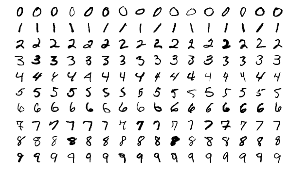
MNIST dataset consists of 70K images of handwritten numbers 0 to 9.

MNIST examples: https://en.wikipedia.org/wiki/MNIST_database

Each image has a size of \(28 \times 28\) and comes with a correct number. In this assignment, we try to classify handwritten images of MNIST using the best approximation.

1. Loading MNIST dataset

After downloading the file attached to the document, extract it. There should be four mat files.

File name	Description
train_image.mat	It’s 60K handwritten images. We are trying to get the best approximate solution using the images in train_image.
train_target.mat	Contains the correct numbers for each image in train_image in order.
test_image.mat	10K handwritten images. Will be used to validate solutions obtained through train_image.
test_target.mat	Correct numbers for test_image.

Enter the following commands in matlab in order to load data into the Workspace. Also, specify the type of each data as double.

load('training_image.mat'); train_x = double(train_x);
load('training_target.mat'); train_y = double(train_y);
load('test_image.mat'); test_x = double(test_x);
load('test_target.mat'); test_y = double(test_y);

Make sure 4 variables are created in the Workspace.

Name          Size                      Bytes  Class  

test_x       28x28x10000             62720000  double              
test_y        1x10000                   80000  double              
train_x      28x28x60000            376320000  double              
train_y       1x60000                  480000  double  

2. Composing and solving Normal equation [Binary classification]

First, let’s find a solution to distinguish only two numbers 0 and 1. Reconstruct the variable by extracting only the data with correct answer numbers 0 or 1.

% find indices whose value is either 0 or 1.
train_idx = [find(train_y == 0), find(train_y == 1)];
test_idx = [find(test_y == 0), find(test_y == 1)];

% Leave only data that are 0 or 1.
train_x = train_x(:, :, train_idx); train_y = train_y(:, train_idx);
test_x = test_x(:, :, test_idx);    test_y = test_y(:, test_idx);

Use the reshape command on train_x to construct a data matrix \(M\) where each row is an image.

M = reshape(train_x, 28^2, [])';    % [] means that 'matche dimension automatically'.
y = train_y';

(Almost trivially) There are no \(y\) that satisfies \(Mx=y\). So we are goint to try to find the best approximate solution.

1. Simply, we can use \ syntax to get the solution. \ will automatically find the most suitable solution.

    x = M \ y;  % the most simple way.
   

   However, in this case \ works quite slowly, and it is difficult to understand how to find a solution at our level.

2. We can also find the solution by directly constructing the normal equation. In this case, the linsolve command is used to find the solution of the linear system.
   (In this case, linsolve uses \(LDU\)-decomposition to find the solution. Also, the syntax \ uses the same algorithm.)

    A = M' * M;
    b = M' * y;
    x = linsolve(A, b);
   

   If you find a solution using the above code, there is a high probability that the obtained solution contains very wrong values. This is because \(A\) is numerically unstable since the elements of \(A\) are generally close to zero, and only very small amounts of elements appear very large. There are many ways to make the \(A\) numerical stable, but here we will use the simplest way which is adding a small noise (perturbation) to \(A\). Of course, the solution obtained in this way is slightly different from the actual value. But let’s ignore small errors here.
   (You don’t have to try to understand this part.)

    A = M' * M + rand(size(M, 2)) * 0.001;  % add random perturbation.
    b = M' * y;
    x = linsolve(A, b);
   

Let’s compare the time required for 1 and 2 respectively.

%% method 1
tic; x = M \ y; toc;
%% method 2
tic;
A = M' * M + rand(size(M, 2)) * 0.001;
b = M' * y;
x = inv(A) * b; 
toc;

3. Solution validation

Create the data matrices \(T\) and \(z\) using the test data reconstructed only with 0 and 1, which were loaded earlier.

T = reshape(test_x, 28^2, [])';
z = test_y';

Calculate the predicted value \(w\) using the solution \(x\) obtained earlier, round it and compare it with the value of \(z\).

w = T * x;   % compute the prediction by the best approximate solution `x`
acc = sum(round(w) == z) / length(w);  % compute the accuracy: (# of correct answers) / (# of data points)
fprintf('Accuracy = %.2f %% \n', acc * 100)

We can see that the classification model(solution \(x\)) is quite accurate with 98% accuary.

4. More classes of numbers

Now let’s classify more numbers. First, specify the numbers we want to classify,

num_for_use = [0, 1, 2, 3];

and then use the `for’-loop to select only the numbers we want to classify. The way is exactly the same as above.

train_idx = [];     % create empty idcies
test_idx = [];
for i = num_for_use
    train_idx = [train_idx, find(train_y == i)];
    test_idx = [test_idx, find(test_y == i)];
end

Now, the rest is the same as in the previous example. The model that classifies the four numbers 0, 1, 2, 3 is about 70% accurate.

Exercises

1. Make a model to classify multiple numbers.

2. Create and validate a model that classifies two numbers 0 and 9 by following the above. In practice, the accuracy should be similar to a model that classifies 0 and 1 (about 98%). How about your result?

   If the result is not the same as you expected, think what is the problem and try to correct it.