Assignment 10

December 3, 2021 7 minute read

과제 10

과제	10
점수	10
기한	12월 9일, 11:59 PM
제출 형식	한개의 매트랩 fig파일 (*.fig)
제출 장소	KLMS assignment 10
파일	Download

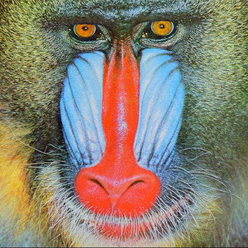
여러분은 우리 교과서의 표지가 어떻게 생겼는지 살펴본 적이 있나요? 표지에 있는 원숭이는 라이온킹의 라피키로 많이 알려져 있는 맨드릴 입니다. 흔히 개코원숭이의 일종으로 알려져있지만, 지금은 긴꼬리원숭이과의 맨드릴속으로 분리되었죠. 중앙의 컬러 이미지는 그렇다 치더라도, 표지의 가장자리를 따라서 점점 흐려지는 흑백 이미지는 무엇을 뜻하는 것일까요?

1. Singular Value Decomposition과 Main Feature

Singular value decomposition(SVD)는 정사각 행렬이 아닌 행렬들에 적용할 수 있는 eigen value decomposition(EVD)의 일반화라고 볼 수 있습니다. 어떤 종류의 행렬이던지에 관계없이, 항상 orthogonal한 vector들과 positive singular value들을 얻을 수 있다는 점에서는 EVD보다 더 강력한 도구라고 볼 수도 있습니다.

설명을 쉽게 하기 위해서 대칭행렬 \(A\)를 생각해보겠습니다. 우리가 행렬 \(A\)의 eigen value들과 eigen vector들을 구했을 때, 가장 큰 eigen value에 대응되는 eigen vector는 “행렬을 ‘잘’ 쪼개서 여러 방향으로 분리했을 때, 행렬 \(A\)를 가장 잘 표현하는 방향”이라고 생각할 수 있을 겁니다. SVD로 구한 singular value들과 singular vector들도 마찬가지로 해석할 수 있습니다. \(A\)의 singular value들을 큰 순서대로

\[\sigma_1 \ge \sigma_2 \ge \cdots \ge \sigma_m,\]

라 하고, 여기에 대응되는 left and right singular vector들을 각각

\[\begin{align*} u_1,\,u_2,\, \cdots,\, u_m\\ v_1,\,v_2,\, \cdots,\, v_n \end{align*}\]

라고 한다면, 우리는 \(A\)를 다음과 같은 rank 1 matrix들의 합으로 나타낼 수 있습니다.

\[A = u_1\sigma_1v_1^T + u_2\sigma_2v_2^T + \cdots + u_r\sigma_rv_r^T, ~~ \mbox{where} ~~ \sigma_k = 0 \quad\mbox{for}\quad k > r.\]

여기서, 값이 충분히 큰 singular value들로 구성된 rank 1 matrix들만 골라서 새로운 행렬 \(\tilde{A}\)를 구성한다면, \(\tilde{A}\)는 원래 \(A\)의 main feature를 대부분 유지하면서 \(A\)보다는 적은 차원의 행렬이 될 것입니다. 즉, \(A\)의 low dimensional approximation이 되는 것이죠.

2. 이미지의 저 차원 근사

위 이미지를 매트랩에 불러온 뒤, SVD를 수행하겠습니다. 이미지를 2차원 행렬로 만들기 위해, rgb2gray명령어를 사용하고, svd명령어를 이용하여 SVD를 수행할 수 있습니다. 이 때, svd명령어는 double형 변수에만 적용 가능하므로, 이미지를 double형으로 바꾸어줍니다.

mandrill = rgb2gray(imread('mandrill.png'));
mandrill = double(mandrill);
[U, S, V] = svd(mandrill);

모든 SV들을 사용하여 이미지를 재결합한 뒤 확인해보겠습니다.

fullSV = U * S * V';
figure; 
subplot(1, 2, 1); 
imshow(mandrill, [0, 255]);
title('Original image');
subplot(1, 2, 2); 
imshow(fullSV, [0, 255]);
title('Using all singular values');

원본 이미지와 완전히 같은 결과를 볼 수 있습니다. 이번에는, 5개의 아주 적은 SV만 선택하여 이미지를 근사해보겠습니다.

SV10 = U(:, 1:5) * S(1:5, 1:5) * V(:, 1:5)';
figure; 
subplot(1, 2, 1); 
imshow(mandrill, [0, 255]);
title('Original image');
subplot(1, 2, 2); 
imshow(SV10, [0, 255]);
title('Using 5 singular values');

오른쪽 그림만 보고 원본이 어떤 이미지인지 알 수 있겠나요? 얼만큼의 SV를 선택해야 충분히 적은 차원의 SV들 만으로, 충분히 보존된 이미지를 얻을 수 있을까요? SV들을 크기순으로 나열해보겠습니다.

figure;
bar(diag(S));
title('Singular values');

가장 큰 100개의 SV만 선택해도, 나머지 400여개의 SV보다는 충분히 커보입니다. 100개의 SV로 이미지를 근사해보겠습니다.

SV100 = U(:, 1:100) * S(1:100, 1:100) * V(:, 1:100)';
figure; 
subplot(1, 2, 1); 
imshow(mandrill, [0, 255]);
title('Original image');
subplot(1, 2, 2); 
imshow(SV100, [0, 255]);
title('Using 100 singular values');

원본과의 차이점을 느낄 수 있나요? 스스로 여러개의 SV를 선택 해가면서 이미지를 근사하고 결과를 확인해보세요.

3. 표지 이미지 만들기

앞의 결과들을 이용해 교과서의 표지를 만들어 보겠습니다.

% load 'mandrill' image and set values into [0, 1].
img = imread('mandrill.png');
img = double(img) / 255;
% make gray image and store.
g_img = rgb2gray(img);
imwrite(g_img, 'img_orig.jpg');

% find SVD of the gray image.
[U, S ,V] = svd(g_img);

% for visualization
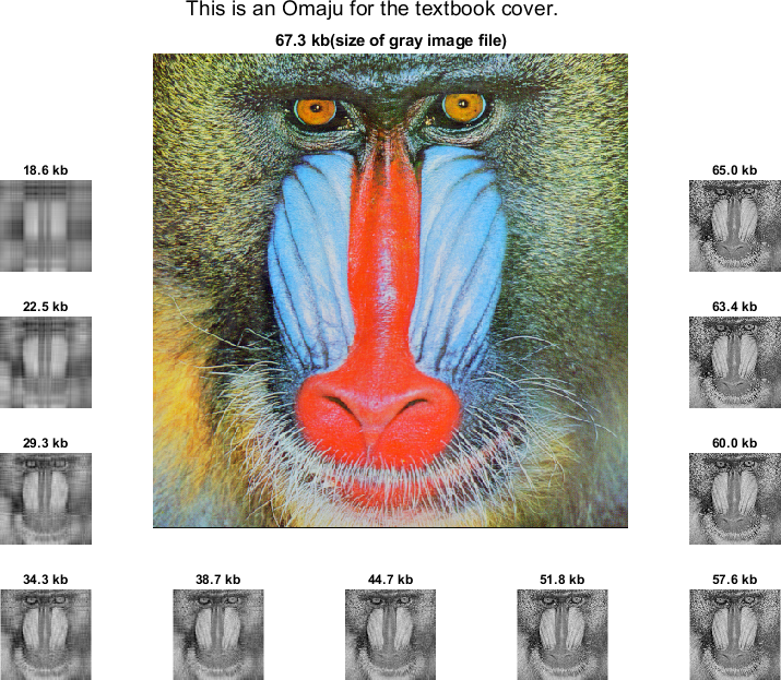
figure;
sgtitle ('This is an Omaju for the textbook cover.')
preset = [200 , 150 , 100 , 80, 50, 30, 20, 15, 10, 5, 3];
fig_loc = [10:5:25 , 24, 23, 22, 21:-5:6];
for i = 1:11
    temp_S = S;
    temp_S(preset(i):end, preset(i):end) = 0;
    temp_img = U * temp_S * V';
    img_name = sprintf('img_%d.jpg', preset(i));
    imwrite (temp_img, img_name);
    subplot (5, 5, fig_loc (i));
    imshow (temp_img);
    title(sprintf('%.1f kb', imfinfo(img_name).FileSize / 1024))
end
% draw 'full' gray image
subplot(5, 5, [2:4, 7:9, 12:14, 17:19]) ; imshow (img);
title(sprintf ('%.1f kb(size of gray image file)', imfinfo ('img_orig.jpg'). FileSize / 1024))

연습문제

첨부된 mat 파일을 다운로드 후, 매트랩에 불어오세요. 작업공간에 변수 I가 생성되어야 합니다.

SVD를 이용해서 I의 rank 1 근사 I_major를 생성하세요. 이 때, I_major는 I의 가장 큰 SV를 이용하여 생성되어야 합니다. 새로운 figure창에 이미지 I_major를 나타낸 뒤, assign10_ex1.fig으로 저장하세요.

제출

연습문제의 1번에서 저장한 assign10_ex1.fig를 KLMS의 지정된 장소에 제출하세요. 제출기한과 점수를 확인하시기 바랍니다.

Assignment 10

Assignment	10
점수	10
기한	Dec 09, 11:59 PM
제출 형식	One MATLAB figure files (*.fig)
제출 장소	KLMS assignment 10
파일	Download

Have you ever looked at what the covers of our textbooks? The monkey on the cover is Mandrill, better known as Rafiki from The Lion King. Commonly known as a species of baboon, but it has now been isolated as Mandrillus in Cercopithecidae. Do you know the meaning of the color image and the gray image faded along the sides of the cover?

1. The Singular Value Decomposition and Main Features

Singular value decomposition (SVD) can be viewed as a generalization of eigen value decomposition (EVD) that can be applied to non-square matrices. It can be seen as a more powerful tool than EVD in that it can always obtain orthogonal vectors and positive singular values, regardless of any kind of matrix.

For ease of explanation, consider the symmetric matrix \(A\). When we obtain the eigen values and eigen vectors of the matrix \(A\), the eigenvector corresponding to the largest eigenvalue can be thought as the “best direction” representing the matrix \(A\) when the matrix is ’well’ partitioned in several directions. Singular values and singular vectors obtained by SVD can also be interpreted in the same way. Let singular values of \(A\) in descending order be

\[\sigma_1 \ge \sigma_2 \ge \cdots \ge \sigma_m,\]

and each of the corresponding left and right singular vectors be

\[\begin{align*} u_1,\,u_2,\, \cdots,\, u_m\\ v_1,\,v_2,\, \cdots,\, v_n \end{align*}.\]

Then we can represent \(A\) as the sum of rank 1 matrices:

\[A = u_1\sigma_1v_1^T + u_2\sigma_2v_2^T + \cdots + u_r\sigma_rv_r^T, ~~ \mbox{where} ~~ \sigma_k = 0 \quad\mbox{for}\quad k > r.\]

Here, if we construct a new matrix \(\tilde{A}\) by selecting only rank 1 matrices composed of sufficiently large singular values, \(\tilde{A}\) can be thought as a main feature of the original \(A\). That is, it becomes a low dimensional approximation of \(A\).

2. Low-dimensional approximation of images

After loading the above image into MATLAB, we will perform SVD. To make an image into a 2D matrix, we will use the rgb2gray command, and perform SVD using the svd command. The svd command is applicable only to double type variables, so we should change the image to double type.

mandrill = rgb2gray(imread('mandrill.png'));
mandrill = double(mandrill);
[U, S, V] = svd(mandrill);

Let’s re-compose the image using all the SVs and check it out.

fullSV = U * S * V';
figure; 
subplot(1, 2, 1); 
imshow(mandrill, [0, 255]);
title('Original image');
subplot(1, 2, 2); 
imshow(fullSV, [0, 255]);
title('Using all singular values');

We can see the exact same result as the original image. This time, we will approximate the image by selecting only smallest 5 SVs.

SV10 = U(:, 1:5) * S(1:5, 1:5) * V(:, 1:5)';
figure; 
subplot(1, 2, 1); 
imshow(mandrill, [0, 255]);
title('Original image');
subplot(1, 2, 2); 
imshow(SV10, [0, 255]);
title('Using 5 singular values');

Can you tell what the original image is just by looking at the image on the right? How many SVs should be selected to obtain a sufficiently preserved image with SVs of sufficiently small dimensions? Let’s list the SVs in order of size.

figure;
bar(diag(S));
title('Singular values');

Even if we choose only the 100 largest SVs, they look bigger enough than the other 400 SVs. Let’s approximate the image with 100 SVs.

SV100 = U(:, 1:100) * S(1:100, 1:100) * V(:, 1:100)';
figure; 
subplot(1, 2, 1); 
imshow(mandrill, [0, 255]);
title('Original image');
subplot(1, 2, 2); 
imshow(SV100, [0, 255]);
title('Using 100 singular values');

Can you find the difference from the original? Try to approximate the image by selecting several SVs yourself and check the result.

3. An omaju of the textbook cover

Let’s make the cover of the textbook using the previous results.

% load 'mandrill' image and set values into [0, 1].
img = imread('mandrill.png');
img = double(img) / 255;
% make gray image and store.
g_img = rgb2gray(img);
imwrite(g_img, 'img_orig.jpg');

% find SVD of the gray image.
[U, S ,V] = svd(g_img);

% for visualization
figure;
sgtitle ('This is an Omaju for the textbook cover.')
preset = [200 , 150 , 100 , 80, 50, 30, 20, 15, 10, 5, 3];
fig_loc = [10:5:25 , 24, 23, 22, 21:-5:6];
for i = 1:11
    temp_S = S;
    temp_S(preset(i):end, preset(i):end) = 0;
    temp_img = U * temp_S * V';
    img_name = sprintf('img_%d.jpg', preset(i));
    imwrite (temp_img, img_name);
    subplot (5, 5, fig_loc (i));
    imshow (temp_img);
    title(sprintf('%.1f kb', imfinfo(img_name).FileSize / 1024))
end
% draw 'full' gray image
subplot(5, 5, [2:4, 7:9, 12:14, 17:19]) ; imshow (img);
title(sprintf ('%.1f kb(size of gray image file)', imfinfo ('img_orig.jpg'). FileSize / 1024))

Exercises

After downloading the attached mat file, load it into MATLAB. Variable I should be created in Workspace.

Create a rank 1 approximation I_major of I using SVD. At this time, I_major should be created using the largest SV of I. Display the image I_major in a new figure window and save it as assign10_ex1.fig.

Submission

Submit the assign10_ex1.fig saved in problem 1 of the exercise to the KLMS. Please check the submission deadline and score.

Share on

Twitter Facebook

MATLAB TA

Assignment 10

과제 10

1. Singular Value Decomposition과 Main Feature

2. 이미지의 저 차원 근사

3. 표지 이미지 만들기

연습문제

제출

Assignment 10

1. The Singular Value Decomposition and Main Features

2. Low-dimensional approximation of images

3. An omaju of the textbook cover

Exercises

Submission

Share on

Leave a comment