
Assignment 1
과제 1
| 과제 | 1 |
|---|---|
| 점수 | 0 |
| 제출 | False |
이 과제는 매트랩을 처음 접하는 사람들에게 도움이 될 몇가지 기본적인 내용들을 담고 있습니다. 매트랩을 아직 설치하지 않았거나, 한번도 열어보지 않았다면 먼저 Intro의 내용을 읽어보길 권장합니다.
이 번 과제는 아무것도 제출할 필요가 없습니다. 내용을 읽어보고, 매트랩을 실행해서 스스로 따라해보는게 과제입니다.
0. Hello world
매트랩에서는 disp명령어로 문자열을 출력합니다.
disp("Hello, world!!");
또는 특정 변수를 출력할 수 있습니다.
s = "hello"; x = exp(1); y = [1, 2, 3; 4, 5, 6];
disp(s); disp(x); disp(y);
disp함수 안에 서로 다른종류의 변수를 동시에 입력할수는 없습니다. 이런 경우, 다른 종류의 변수들을 []로 묶으면 매트랩이 자동으로 형변환을 거친 결과를 출력합니다.
s = "hello"; x = exp(1);
disp(s, y);          % 잘못된 구문
disp([s, y]);        % 가능한 구문
C, C++ 또는 Python등에 익숙한 경우에는, disp함수가 다소 답답하게 느껴질 수 있습니다. 문자열이나 행렬등을 간편하게 출력할수는 있지만, 단순히 문자열을 출력하는 용도로만 사용하기엔 기능이 한정적입니다. 사실, 매트랩에서는 또다른 출력함수인 fprintf를 사용할 수 있습니다. fprintf의 기능은 C의 printf나 Python의 print와 유사합니다.
hw = "Hello, world!!";
times = 14;
fprintf("I am saying '%s' the %03dth time.\n", hw, times);
-
(
sprintf와disp)앞서 소개한 것 처럼
fprintf함수를 이용하면 문자열을 원하는대로 조정하여 출력할 수 있습니다.sprintf와disp함수를 이용해서 만들어낼 수도 있습니다.hw = "Hello, world!!"; times = 14; s = sprintf("I am saying '%s' the %03dth time.\n", hw, times); disp(s);
1. 행렬 만들기
매트랩은 행렬계산 및 수치계산에 최적화 된 언어입니다. 행렬계산을 하려면 먼저 매트랩에서 행렬을 어떻게 만드는지를 알아야겠죠? 기본적인 내용은 Week1에 다루었으니, 여기서는 결과만 표시해보겠습니다.
(이번 절에서 부터는 결과를 바로바로 확인하고 싶은 줄에는 ;를 생략하겠습니다.)
% Vectors
x = [1, 2, 3]                       % 1 x 3 vector [1, 2, 3]
y = [1; 2; 3]                       % 3 x 1 vector [1, 2, 3]^T
z = y'                              % transpose of 3 x 1 vector y (=x)

% Matricies
A = [1, 2, 3; 4, 5, 6; 7, 8, 9]     % 3 x 3 matrix
B = [1, 2; 3, 4; 5, 6]              % 3 x 2 matrix
C = [1, 3, 5; 2, 4, 6]'             % transpose of 2 x 3 matrix (=B)
이런식으로 벡터와 행렬을 직접 입력할 수 있습니다. 또한 특정한 행렬들은 매트랩 명령어를 통해 만들어낼 수도 있습니다. zeros, ones, eye명령어들은 각각 0 행렬, 0 행렬 + 1, 단위행렬(또는 대각선이 1인 행렬)을 생성해줍니다.
% zeros
Z1 = zeros(3)       % 3 x 3 zero matrix
Z2 = zeros(2, 5)    % 2 x 5 zero matrix
z = zeros(1, 3)     % 1 x 3 zero vector

% ones
O1 = ones(2)        % 2 x 2 matrix whose all entries are 1
O2 = ones(2, 3)     % 2 x 3 matrix whose all entries are 1

% eye
I1 = eye(6)         % the identity matrix in R^6
I2 = eye(3, 5)      % 3 x 5 matrix whose main diagonal entries are 1
rand함수를 이용하면 임의의 행렬을 생성할 수도 있습니다.
A = rand(3, 5)              % 3 x 5 random matrix
B = randi([-3, 4], 2, 4)    % 2 x 4 random matrix whose entries are
                            % integers sampled on the interval [-3, 4].
2. 행렬의 계산
여러분은 아마 이전 자료들에서 행렬의 계산에 대한 부분을 보았을 겁니다. 또한 reduced row echelon form을 구해주는 rref를 사용하는 것과, 역행렬을 구하기 위해 inv함수나 A^(-1)등의 구문을 사용하는 걸 이미 알고 있을거에요. 하지만 행렬의 계산은 앞으로의 학습 과정에 매우 중요한 부분인 만큼 다시한번 짚고 넘어가겠습니다.
-
행렬의 수학적 연산
+,*,^,inv매트랩은 기본적으로 실제 수학 연산과 같은 구문을 사용합니다. 다음 코드의 결과들을 손으로 한 계산과 비교해보세요.
(inv와^(-1)은 완전히 같은 결과를 줍니다.)A = [5, 3, -4; 2, -1, 2; 3, 2, -5]; B = [4, -2, 0; 3, 1, 1; 5, -2, -3]; SUM = A + B PROD = A * B POW = A^2 INV = A^(-1) INV2 = inv(A)행렬간 나눗셈은 정의되지 않습니다. 따라서,
A/B와 같은 구문은 수학적으로는 정의할 수 없는 계산입니다. 그렇다면 다음과 같은 계산을 하면 오류 메시지가 나타날까요?DIV = A / B오류 메시지가 나타나지 않고, 무언가 결과를 얻었다면 정상적으로 작동한 것이에요. 관련된 내용은 아래에서 다루겠습니다.
-
역행렬과 계산
일반적인 행렬계산에서, 역행렬 그 자체가 필요해서
A^(-1)을 사용하는 경우는 많지 않습니다. 우리는 일반적으로 \(Ax = b\)와 같은 linear system을 푸는 법을 고민하는데, \(A\)가 non-singular한 경우에는 system의 해를 구하고자 \(x = A^{-1}b\)와 같은 연산을 합니다. 선형대수학을 공부하다 보면, 행렬의 역행렬을 직접 구하기 보다는, 역행렬과 다른 행렬이 곱해진 형태가 필요한 경우가 많이 있습니다. 따라서 매트랩에서는 이런 경우에 사용할 수 있는 구문이 따로 마련되어 있습니다.A = rand(3); % random 3 x 3 matricies A and B B = rand(3); inv_A = inv(A); % inverse of A I1 = inv_A * B I2 = A \ B위에서
I1과I2는 같은 결과를 주는 걸 알수있습니다. 즉,A\B는inv(A)*B대신 쓸 수 있는 구문입니다.이제 위에서
A/B가 어떻게 결과를 줬는지 알겠나요?A/B는A*inv(B)와 혼용해서 쓸 수 있습니다. -
행렬 요소별 연산
.*,.^,./1번에서 굳이 ‘수학적’이라는 용어를 쓴 이유는 무엇일까요? 행렬과 같은 array 구조를 사용하여 계산할때, 행렬의 ‘수학적 연산’이 아닌 ‘요소별 연산’을 사용하는 경우가 아주 많이 때문입니다. 실제로 매트랩과 비슷한 고차원 언어인 Python같은 경우는 기본 연산 구문인
\[A = \begin{bmatrix} a_{11} & a_{12} \\ a_{21} & a_{22} \end{bmatrix}, \quad B = \begin{bmatrix} b_{11} & b_{12} \\ b_{21} & b_{22} \end{bmatrix} ~ \Rightarrow ~ A \star B = \begin{bmatrix} a_{11} \star b_{11} & a_{12} \star b_{12}\\ a_{21} \star b_{21} & a_{22} \star b_{22}\\ \end{bmatrix}\]*,/등이 요소별 연산을 뜻합니다. \(\star\)를 임의의 요소별 연산이라고 했을때, 두 행렬 \(A\)와 \(B\)의 요소별 연산은 다음과 같이 정의할 수 있습니다.다음 코드의 결과들을 손으로 한 계산과 비교해보세요.
 A = [5, 3, -4; 2, -1, 2; 3, 2, -5];
 B = [4, -2, 0; 3, 1, 1; 5, -2, -3];

 SUM = A + B         % naturally elementwise
 EL_PROD = A .* B    % elementwise product
 EL_DIV = A ./ B     % elementwise division
 EL_POW = A.^2       % elementwise power
 EL_INV = A.^(-1)    % elementwise "reciprocal"
행렬의 요소별 연산은 많은 프로그래밍 계산 영역에서 ‘기준’이 되는 연산입니다. 실제로, 매트랩에서 제공하는 수학적 함수들은 요소별로 적용되도록 만들어져 있습니다.
 A = [0, pi/2, pi; -1, 0, 1]
 S = sin(A)          % S = [sin(0), sin(pi/2), sin(pi);
                     %     sin(-1), sin(0), sin(1)]
3. 함수 값 계산
2절의 ‘요소별 계산’을 이용하면 여러가지 함수들의 값을 쉽게 계산할 수 있습니다. 예를들어, \(-3 \le x \le 3\)와 같은 영역에서 \(\sin(x)\)의 값을 구하는 것을 생각해봅시다.
x = [-3, -2, -1, 0, 1, 2, 3];
y = sin(x);
disp(y)
y에는 x의 각 요소에 대한 \(\sin\)함수 값이 들어있습니다. 다시 말하면, 영역 \(-3 \le x \le 3\)의 정수점들에 대한 \(\sin\)함수의 값들이 y입니다.
4. 함수의 그래프 그리기
매트랩의 plot함수를 이용하면 2차원 axis위에 y=sin(x)의 그래프를 그릴 수 있습니다.
x = [-3, -2, -1, 0, 1, 2, 3];
y = sin(x);
plot(x, y)
Result.
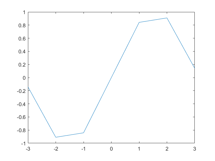
위에서 \(\sin\)값은 정수 grid위에서만 계산되었기 때문에, 결과로 나타나는 그래프는 다소 이상해보입니다. 매트랩의 x0:step:x1구문이나 linspace함수를 이용해서 더 조밀한 \(x\)값들에 대한 \(\sin\)함수 값과 그래프를 그릴 수 있습니다.
x1 = -3:0.1:3;              % x1 = [-3, -2.9, -2.8, ..., 3]
                            % 0.1 is the step size.
x2 = linspace(-3, 3, 200);  % x2 is partition of [-3, 3]
                            % whose length(x2)=200.
y1 = sin(x1); y2 = sin(x2);
plot(x1, y1, x2, y2);       % draw two graphs y1 and y2, simultaniously.
Result.
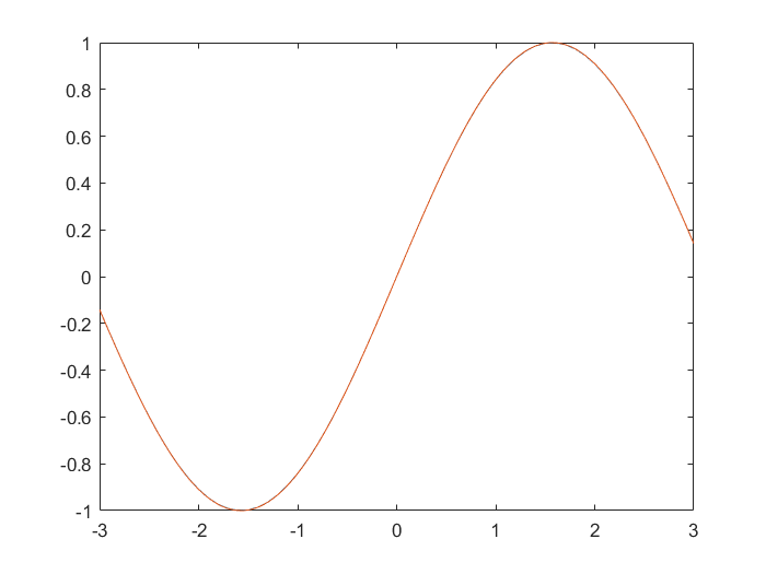
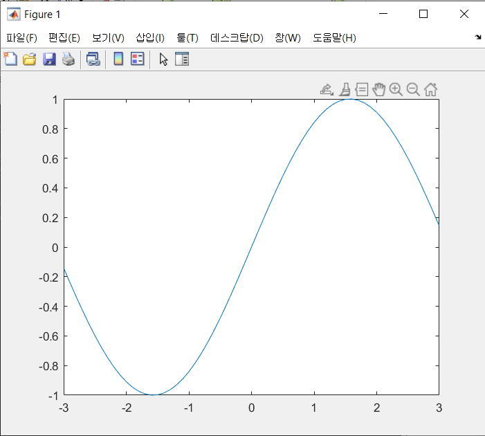
위 결과는, 눈으로 보기에는 하나의 선처럼 보이지만 실제로는 두개의 sine곡선이 겹쳐져 보이는 것입니다. 이럴때는, figure명령어를 이용해서 서로 다른 여러개의 figure window를 생성할 수 있습니다.
figure(1); % open figure 1
plot(x1, y1); % draw y1 in the figure 1
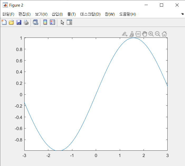
figure(2); % open figure 2
plot(x2, y2); % draw y2 in the figure 2
% you don't have to assign number of figure.
% they will be automatically assigned.
Result.
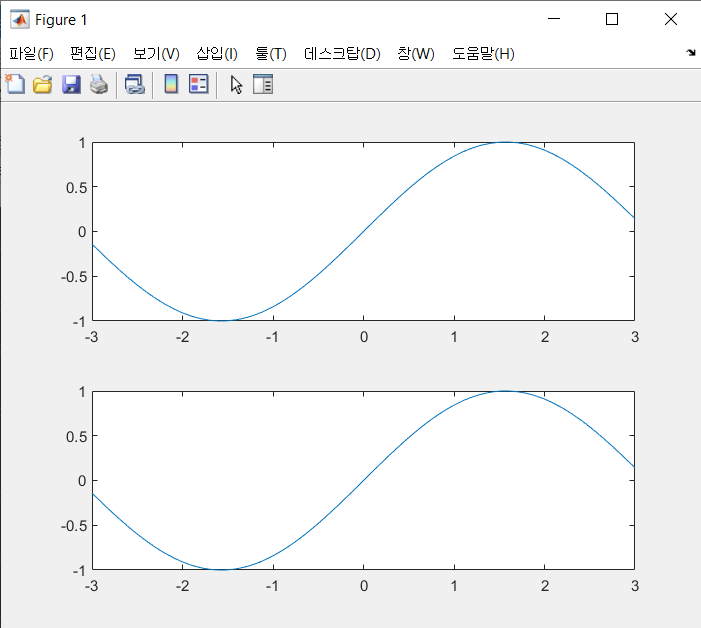
혹은, subplot명령어를 이용해서 한 figure에 여러개의 axis를 그릴 수 있습니다.
figure();
subplot(2, 1, 1);   % make 2 x 1 array of axes and choose the 1st one
plot(x1, y1)

subplot(2, 1, 2);   % choose the 2nd axis
plot(x2, y2)
Result.
이와같이 매트랩을 이용해 여러가지 함수의 값을 구하고, 그래프를 그릴 수 있습니다.
연습문제
-
주어진 범위에서, 함수\(p(x)\)의 그래프를 그리세요.
\[p(x) = x^3 - x, \quad -3 \le x \le 3.\]grid함수를 이용해서 axis의 grid를 표시하세요. -
매트랩 함수
subplot을 이용하여, 하나의 figure window안에 다음 함수들의 그래프를 모두 그리세요.1) \(f_1(x) = |x-1|, \quad -3 \le x \le 3\),
2) \(f_2(x) = \sqrt{|x|}, \quad -4 \le x \le 4\),
3) \(f_3(x) = e^{-x^2}, \quad -4 \le x \le 3\),
4) \(f_4(x) = \frac{1}{10x^2 + 1}, \quad -2 \le x \le 2\).매트랩의
abs,sqrt,exp함수들을 이용해야 할 수도 있습니다.
Assignment 1
| Assignment | 1 |
|---|---|
| Score | 0 |
| Submission | False |
This assignment contains some basic information that will be helpful to those who are new to MATLAB. If you haven’t installed MATLAB yet, or even haven’t opened it, it is recommended to read the contents of Intro.
You do not need to submit anything for this assignment, just read the contents, run MATLAB and follow along.
0. Hello world
In MATLAB, a string is printed with the disp command.
disp("Hello, world!!");
Or you can print out a specific variable.
s = "hello"; x = exp(1); y = [1, 2, 3; 4, 5, 6];
disp(s); disp(x); disp(y);
You cannot enter different kinds of variables in the disp function at the same time. In this case, if you group other kinds of variables with [], MATLAB automatically outputs the result of casting.
s = "hello"; x = exp(1);
disp(s, x);          % Wrong syntax
disp([s, x]);        % Possible syntax
If you are familiar with C, C++, or Python, the disp function can feel a bit frustrating. You can print strings or matrices easily, but the function is limited to use it only for printing strings. In fact, in MATLAB you can use another printing function, fprintf. The function, fprintf, is similar to printf in C and print in Python.
hw = "Hello, world!!";
times = 14;
fprintf("I am saying '%s' the %03dth time.\n", hw, times);
-
(
sprintfanddisp)As previously introduced, the
fprintfcan be used to adjust and print a string as desired. The same thing can also be achieved usingsprintfanddispfunctions.hw = "Hello, world!!"; times = 14; s = sprintf("I am saying '%s' the %03dth time.\n", hw, times); disp(s);
1. Create a matrix
MATLAB is a language optimized for matrix and numerical calculation. To do matrix calculation, you first need to know how to create a matrix in MATLAB, right? Since we covered the basics in Week1, we will only display the results here.
(From this section, we will omit some ; in the line to check the result immediately.)
% Vectors
x = [1, 2, 3]                       % 1 x 3 vector [1, 2, 3]
y = [1; 2; 3]                       % 3 x 1 vector [1, 2, 3]^T
z = y'                              % transpose of 3 x 1 vector y (=x)

% Matricies
A = [1, 2, 3; 4, 5, 6; 7, 8, 9]     % 3 x 3 matrix
B = [1, 2; 3, 4; 5, 6]              % 3 x 2 matrix
C = [1, 3, 5; 2, 4, 6]'             % transpose of 2 x 3 matrix (=B)
You can directly enter vectors and matrices in this way. Also, certain matrices can be created via MATLAB commands. The commands zeros, ones, and eye generate zero matrix, zero matrix + 1, and identity matrix (or matrix with diagonal 1), respectively.
% zeros
Z1 = zeros(3)       % 3 x 3 zero matrix
Z2 = zeros(2, 5)    % 2 x 5 zero matrix
z = zeros(1, 3)     % 1 x 3 zero vector

% ones
O1 = ones(2)        % 2 x 2 matrix whose all entries are 1
O2 = ones(2, 3)     % 2 x 3 matrix whose all entries are 1

% eye
I1 = eye(6)         % the identity matrix in R^6
I2 = eye(3, 5)      % 3 x 5 matrix whose main diagonal entries are 1
You can create random matrix using rand function.
A = rand(3, 5)              % 3 x 5 random matrix
B = randi([-3, 4], 2, 4)    % 2 x 4 random matrix whose entries are
                            % integers sampled on the interval [-3, 4].
2. Matrix operation
You’ve probably seen the part about matrix operation in previous materials. Also, you may already know that you use rref to get the reduced row echelon form, and you use syntax like inv or A^(-1) to get the inverse matrix. However, since matrix calculation is a very important part of the learning MATLAB, we will go over it again.
-
Mathematical operations
+,*,^,invBasically, MATLAB uses the same syntax as real math operations. Compare the results of the following code with the calculations done by hand.
(invand^(-1)give exactly the same result.)A = [5, 3, -4; 2, -1, 2; 3, 2, -5]; B = [4, -2, 0; 3, 1, 1; 5, -2, -3]; SUM = A + B PROD = A * B POW = A^2 INV = A^(-1) INV2 = inv(A)The division between matrices is undefined. So, syntax like
A/Bare mathematically indefinable calculations. If so, would you get an error message when you make the following calculations?DIV = A / BIf you don’t see an error message and you get something, it’s working fine. Related content will be covered below.
-
Inverse matrix and computaions
In general matrix calculations, it is not common to use
A^(-1)to get the inverse matrix itself. When we consider how to solve a linear system such as \(Ax = b\), if \(A\) is non-singular then we perform the operations like \(x = A^{-1}b\). When we studying linear algebra, there are many cases where we need a form in a multiplication of inverse matrix and other matrices, rather than directly obtaining the inverse matrix. Therefore, in MATLAB, there is a syntax that can be used in this case.A = rand(3); % random 3 x 3 matricies A and B B = rand(3); inv_A = inv(A); % inverse of A I1 = inv_A * B I2 = A \ BAbove, you can see that
I1andI2give the same result. In other words,A\Bis a syntax that can be used instead ofinv(A)*B.Now do you see how
A/Bgave the result in the previous part?A/Bcan be used interchangeably withA*inv(B). -
Element-wise operations
.*,.^,./Guess why do we use the term ‘mathematical’ in the number 1? This is because when we calculate using an array structure such as a matrix, there are many cases where ‘element-wise operation’ is used rather than’mathematical operation’ of the matrix. In fact, in the case of Python, a high level language similar to MATLAB, the basic syntax
\[A = \begin{bmatrix} a_{11} & a_{12} \\ a_{21} & a_{22} \end{bmatrix}, \quad B = \begin{bmatrix} b_{11} & b_{12} \\ b_{21} & b_{22} \end{bmatrix} ~ \Rightarrow ~ A \star B = \begin{bmatrix} a_{11} \star b_{11} & a_{12} \star b_{12}\\ a_{21} \star b_{21} & a_{22} \star b_{22}\\ \end{bmatrix}\]*and/means element-wise operation. Assuming that \(\star\) is an arbitrary element-wise operation, the element-wise operation of the two matrices \(A\) and \(B\) can be defined as follows.Compare the results of the following code with the calculations done by hand.
 A = [5, 3, -4; 2, -1, 2; 3, 2, -5];
 B = [4, -2, 0; 3, 1, 1; 5, -2, -3];

 SUM = A + B         % naturally elementwise
 EL_PROD = A .* B    % elementwise product
 EL_DIV = A ./ B     % elementwise division
 EL_POW = A.^2       % elementwise power
 EL_INV = A.^(-1)    % elementwise "reciprocal"
Element-wise operations of matrices are a ‘standard’ in many areas of programming computation. Actually, the mathematical functions provided by MATLAB are designed to be applied in element-wise.
 A = [0, pi/2, pi; -1, 0, 1]
 S = sin(A)          % S = [sin(0), sin(pi/2), sin(pi);
                     %     sin(-1), sin(0), sin(1)]
3. Compute function values
You can easily calculate the values of various functions by using the’element-wise calculation’ in Section 2. For example, consider evaluating the value of \(\sin(x)\) in the interval \(-3 \le x \le 3\).
x = [-3, -2, -1, 0, 1, 2, 3];
y = sin(x);
disp(y)
y contains the value of the \(\sin\) function for each element of x. In other words, the values of the \(\sin\) function for the integer points in the range \(-3 \le x \le 3\) are y.
4. Draw a graph of function
Using MATLAB’s plot function, you can draw a graph of y=sin(x) on a 2D axis.
x = [-3, -2, -1, 0, 1, 2, 3];
y = sin(x);
plot(x, y)
Result.
However, the \(\sin\) value above was calculated only on the integer grid. Thus the resulting graph looks a bit strange. You can use MATLAB’s x0:step:x1 syntax or linspace function to get more fine grid for \(x\) and plot the values and graphs of the \(\sin\) function on that.
x1 = -3:0.1:3;              % x1 = [-3, -2.9, -2.8, ..., 3]
                            % 0.1 is the step size.
x2 = linspace(-3, 3, 200);  % x2 is partition of [-3, 3]
                            % whose length(x2)=200.
y1 = sin(x1); y2 = sin(x2);
plot(x1, y1, x2, y2);       % draw two graphs y1 and y2, simultaniously.
Result.
The result above is that it looks like a single line to the eye, but actually two sine curves overlap. In this case, you can create several different figure windows using the figure command.
figure(1);          % open figure 1
plot(x1, y1);       % draw y1 in the figure 1

figure(2);          % open figure 2
plot(x2, y2);       % draw y2 in the figure 2

% you don't have to assign number of figure.
% they will be automatically assigned.
Result.
Alternatively, you can draw multiple axes on one figure using the subplot command.
figure();
subplot(2, 1, 1);   % make 2 x 1 array of axes and choose the 1st one
plot(x1, y1)

subplot(2, 1, 2);   % choose the 2nd axis
plot(x2, y2)
Result.
Now, you can calculate the values of various functions and draw graphs using MATLAB.
Exercises
-
For a given interval, plot the function \(p(x)\). Use the
\[p(x) = x^3 - x, \quad -3 \le x \le 3.\]gridfunction to display the grid of the axis. -
Using the MATLAB function
subplot, plot all of the following functions in a single figure window.1) \(f_1(x) = |x-1|, \quad -3 \le x \le 3\),
2) \(f_2(x) = \sqrt{|x|}, \quad -4 \le x \le 4\),
3) \(f_3(x) = e^{-x^2}, \quad -4 \le x \le 3\),
4) \(f_4(x) = \frac{1}{10x^2 + 1}, \quad -2 \le x \le 2\).You may have to use MATLAB `abs`, `sqrt` and `exp` functions.
Leave a comment