Assignment 2

과제 2

과제	2
파일	Download
점수	8
기한	Sep 30, 11:59 PM
제출 형식	두개의 매트랩 fig파일 (*.fig)
제출 장소	KLMS assignment 2

지난 과제 1에서 1차원 함수의 그래프를 그리는 법을 다뤘습니다. 이번에는 지난 과제에 이어서, 매트랩을 이용한 시각화 방법들에 대해 설명합니다.

0. 연습문제 해설

지난 시간의 연습문제를 다시 읽어보겠습니다.

1. 주어진 범위에서, 함수\(p(x)\)의 그래프를 그리세요. grid함수를 이용해서 axis의 grid를 표시하세요.

   \[p(x) = x^3 - x, \quad -3 \le x \le 3.\]

   ---

   처음 등장한 grid함수를 제외하면, 1 번의 내용은 그리 어렵지 않았을 것이라고 생각합니다. 매트랩에서 figure와 plot을 이용해 그래프를 그리면, 그래프의 격자를 따로 표시하지 않고 그래프를 그려줍니다. grid명령어를 사용하면 좌표축의 그리드를 선으로 표시할 수 있어요.

   MATLAB codes

    % assignment1_ex1
   
    x = linspace (-3 , 3 , 500) ; % Construct a vector x
    p = x.^3 - x;       % Construct a vector p
   
    figure;             % Make a new figure
    subplot(2, 1, 1)    % make a 2 x 1 axis grid and choose 1st
    plot(x, p);         % Draw the graph
    title("Plotting graph without grid lines");
   
    subplot(2, 1, 2)    % choose 2nd axis
    plot(x, p);         % Draw the graph
    grid on;            % draw grid lines
    title("Plotting graph with grid lines");
   

   MATLAB results

   

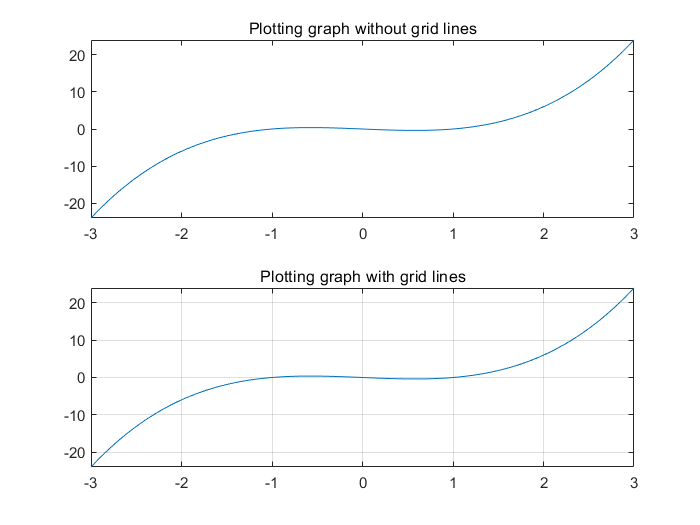
   title명령어를 이용해 axis의 제목을 설정한 것에도 주목하세요.

2. 매트랩 함수 subplot을 이용하여, 하나의 figure window안에 다음 함수들의 그래프를 모두 그리세요.

   1) \(f_1(x) = |x-1|, \quad -3 \le x \le 3\),
   2) \(f_2(x) = \sqrt{|x|}, \quad -4 \le x \le 4\),
   3) \(f_3(x) = e^{-x^2}, \quad -4 \le x \le 3\),
   4) \(f_4(x) = \frac{1}{10x^2 + 1}, \quad -2 \le x \le 2\).

   매트랩의 abs, sqrt, exp함수들을 이용해야 할 수도 있습니다.

   ---

   2번 문제 역시, 지난 시간의 내용을 참고하면 쉽게 해결할 수 있습니다.

   MATLAB codes

    % assignment1_ex2
   
    figure; % Open a new figure window.
   
    %% i. f(x) = |x -1| for -3 <= x <= 3.
    subplot(2, 2, 1) ;      % Make a subplot in a figure window .
    x = -3:0.01:3;          % Construct a linearly - spaced vector x.
    plot(x, abs(x - 1)) ;   % Plot the function f(x)
                            % over the specified domain x.
    axis tight;             % Axis limits to the range of the data .
    title ('(1)');
   
    %% ii. f(x) = sqrt (|x|) for -4 <= x <= 4.
    subplot(2, 2, 2);
    x = -4:0.01:4;
    plot(x, sqrt(abs(x)));
    axis tight;
    title('(2)');
   
    %% iii. f(x) = exp( -x^2) for -4 <= x <= 4.
    subplot(2, 2, 3);
    x = -4:0.01:4;
    plot(x, exp(-x.^2));
    axis tight;
    title('(3)');
   
    %% iv. f(x) = 1/(10* x^2 + 1) for -2 <= x <= 2.
    subplot(2, 2, 4);
    x = -2:0.01:2;
    plot(x, 1./(10 * x.^2 + 1));
    axis tight;
    title('(4)');
   

   MATLAB results

   

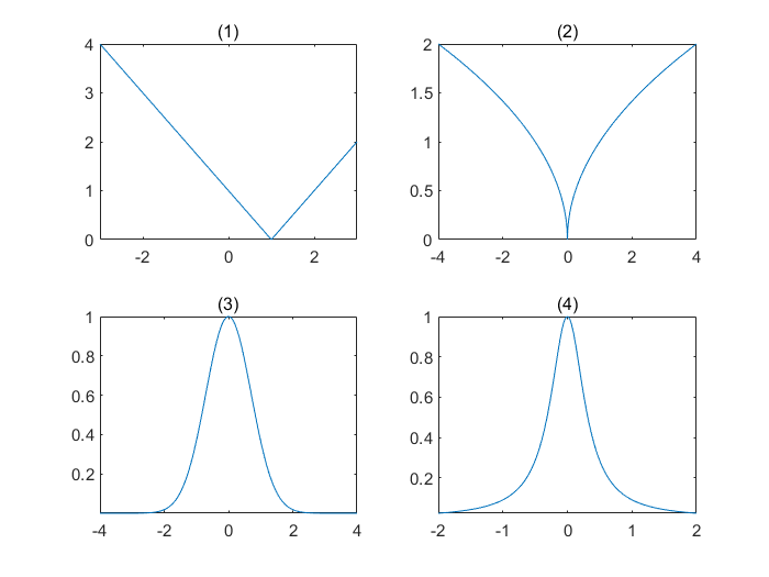
   axis명령어를 이용하면 좌표축의 범위를 세부적으로 조절할 수 있습니다. 스스로 여러 옵션들을 시험해보세요.

1. 극좌표의 그래프

plot명령어는 2차원 좌표계 중에서도 우리에게 가장 익숙한 직교좌표계, 즉

\[e_1 = \begin{bmatrix} 1 & 0 \end{bmatrix}^T,\quad e_2 = \begin{bmatrix} 0 & 1 \end{bmatrix}^T\]

들로 span되는 선형공간상에 그래프를 그려주는 명령어입니다. 하지만, 우리가 잘 아는 또 다른 좌표계인 극좌표계에 그래프를 그리려면 어떻게 해야할까요? 다음과 같은 함수를 생각해봅니다.

\[r = 3 - 3\cos\theta\ -\ 3\sin\theta.\]

plot명령어를 이용해서 그래프를 그린다면 다음과 같이 나타날 것입니다.
(직접 결과를 확인해보세요.)

MATLAB codes

theta = -pi:0.01:pi;
r = 3 - 3 * cos(theta) - 3 * sin(theta);

figure();
plot(theta, r);
title('Using `plot`'); grid on; axis tight;

이번에는 극좌표상에 그래프를 그려주는 polar명령어를 이용해서 그려보겠습니다. polar명령어의 사용법은 plot과 대동소이합니다. 단지 그래프를 그리는 좌표축이 달라지는 것 뿐이에요.

MATLAB codes

theta = -pi:0.01:pi;
r = 3 - 3 * cos(theta) - 3 * sin(theta);

figure();
polar(theta, r);
title('Using `polar`'); grid on; axis tight;

2. 매개변수 함수의 그래프

앞선 예제에서는 \(y=f(x)\)또는 \(r = g(\theta)\)와 같은 ‘음함수’의 형태로 나타낼 수 있는 함수들을 다루었습니다. 음함수의 형태로는 나타내기 어려운 함수들의 경우, 우리는 주로 매개변수를 이용해 함수를 표현하게 됩니다.

\[x = \sin(t), \quad y = \cos(t), \quad -\pi \le t \le \pi.\]

MATLAB codes

t = -pi:0.01:pi;
x = sin(t);
y = cos(t);

figure();
plot(x, y);
title('parametric circle'); grid on; axis tight;

사실 여러분들은 이미 매개 변수 함수에 대해서 배운적이 있습니다. 고등학교때 배운, 3차원 좌표축에서 직선의 방정식을 나타낼 때 매개변수를 이용하여 얻어낸 수식을 사용하였습니다.

\[\begin{matrix} x &=& 3t\\ y &=&-2t\\ z &=& t \end{matrix}, \quad t\in\mathbb{R} \quad \Longleftrightarrow \quad (3t,\,-2t,\,t) \quad \Longleftrightarrow \quad \frac{x}{3} = -\frac{y}{2} = z.\]

매트랩에서 3차원 공간상에 매개변수 함수의 그래프를 그리는 방법은 plot3를 이용하는 것입니다.

MATLAB codes

t = -10:0.01:10;
x = 3 * t;
y = -2 * t;
z = t;

figure();
plot3(x, y, z);
title('3D line'); grid on; axis tight;

이전에 본 plot과는 달리 plot3명령어는 3차원 \(xyz\)-좌표축에 그래프를 그려줍니다. 직선 뿐만 아니라, 3차원 곡선도 역시 plot3명령어를 이용하여 그릴 수 있습니다. 다음 매개변수 함수를 생각해보면,

\[c(t) = \left(t\cos(20\pi t), t\sin(20\pi t), \tanh(\pi t)\right), \quad -1 \le t \le 1,\]

\(c\)는 3차원 좌표축에서 원점을 중심으로 뻗어나가는 helix를 표현하게 될 것입니다.

MATLAB codes

t = -1:0.001:1;
x = t .* cos(20 * pi * t);
y = t .* sin(20 * pi * t);
z = tanh(pi * t);

figure();
plot3(x, y, z);
title('3D helix curve, c(t) = (tcos(20\pit), tsin(20\pit), tanh(\pit))');
grid on; axis tight;

이 때, 벡터들간의 요소별 연산에는 *이 아닌 .*가 쓰였다는 점 유의하세요.

3. 3차원 곡면 나타내기

다음 방정식을 생각해 보겠습니다.

\[z = xe^{-x^2 - y^2}, \quad -2 \le x \le 2,~-2 \le y \le 2.\]

앞선 예시들과는 달리, 이 방정식의 그래프는 단순히 선으로 나타낼 수 없다는 걸 금방 알 수 있을겁니다. 1차원 함수의 그래프와, 매개변수를 이용한 곡선의 방정식은 1차원 그래프(선 또는 곡선)를 가지기 때문에 x1:step:x2나 linspace함수를 이용해서 함수의 범위를 표현할 수 있었습니다. 하지만, 곡면의 그래프는 선보다 높은 차원의 객체이기 때문에, 표현하려면 다른방법이 필요합니다. 처음 함수의 그래프를 배울때로 돌아가보죠. \(y = x^2\)의 그래프를 그리기 위해, \(x\)축위의 점들에 대응되는 \(y\)값들을 계산하고, \((x,\,y)\)점들을 찍은뒤 선으로 잇는 방식을 사용했습니다. 만약 \(z = x^2 + y^2\)의 그래프를 그리기위해 비슷한 작업을 한다면, 적당한 영역안의 모든 \((x,\, y,\, z)\)점들을 찍은 뒤에 그 점들을 모두 덮는 곡면을 주어진 방정식의 그래프로 생각할 수 있을 것이에요. 여기서 ‘적당한 영역안의 모든 \((x,\, y,\, z)\)점들’을 표현하기 위해서는 벡터가 아닌 행렬을 사용해야 합니다. meshgrid함수는 각 좌표축으로의 벡터들을, 영역을 모두 표현하는 행렬들로 바꾸어주는 역할을 합니다.

MATLAB codes

x = 1:5;                    % make an equally spaced vectors x, y
y = -2:2;                   % here, the syntax `-2:2` is equal to `-2:1:2`
[X, Y] = meshgrid(x, y)     % find 2D grid points w.r.t. x and y

MATLAB results

X =

     1     2     3     4     5
     1     2     3     4     5
     1     2     3     4     5
     1     2     3     4     5
     1     2     3     4     5


Y =

    -2    -2    -2    -2    -2
    -1    -1    -1    -1    -1
     0     0     0     0     0
     1     1     1     1     1
     2     2     2     2     2

위 결과에서 볼 수 있듯이, \(X\), \(Y\)는 \(x\), \(y\)로 표현되는 사각형영역 \(\{(x,\, y): 1 \le x \le 5, -2 \le y \le 2\}\)에서의 각 점들에 대한 \(x\), \(y\)값들을 나타내고 있습니다. meshgrid함수를 통해서 1차원으로 표현되는 영역을 2차원으로 확장할 수 있는 것이죠. 이제 우리는 방정식 \(z = xe^{-x^2 - y^2}\)가 나타내는 그래프을 그릴 수 있습니다.

MATLAB codes

x = -2:0.1:2; y = x;
[X, Y] = meshgrid(x, y);
Z = X .* exp(-X.^2 -Y.^2);

figure();
subplot(1, 2, 1)
surf(X, Y, Z);          % draw a surface using `surf` command
axis tight; grid on;
title('Using `surf`command')
subplot(1, 2, 2)
mesh(X, Y, Z);          % draw a surface using `mesh` command
title('Using `mesh`command')
axis tight; grid on;

3차원 곡면을 그리는 명령어에는 surf와 mesh등이 있습니다. 둘의 차이점을 확인해보세요.

• 3차원 곡면을 표현하는 여러가지 방법들

  위에서 설명한 meshgrid, surf, mesh등을 제외하고도 ndgrid, .*, surface등 여러가지 다른 명령어들을 이용해서 3차원 곡면의 그래프를 그릴 수 있습니다. 하지만 곡면이 표현되는 방법은 여기서 설명한것과 같으니 스스로 다른 방법들을 시험해보시기 바랍니다.

---

연습문제

1. 다운로드한 MAS109_assign2_ex1.p을 매트랩의 현재폴더에 위치시킨 뒤에, 지난 과제와 같이 본인의 학번을 input으로 작동시키세요.

    MAS109_assign2_ex1(20210000);
   

   이전까지의 내용을 참고하여, 실행을 통해 얻은 매개변수 방정식의 그래프를 그리는 매트랩 코드를 작성하세요. 그래프가 담긴 매트랩 figure window를 ex1_<studenID>.fig파일로 저장합니다. 다음 명령어를 이용하거나, figure window의 save버튼을 클릭해서 저장할 수 있습니다.

    savefig('ex1_20210000')
   

   현재폴더에 ex1_<studenID>.fig가 생성되었는지 확인하세요. 실행했을때 그래프가 그려진 figure window가 나타나면 정상적으로 저장된 것입니다.

   • 그래프는 2차원 \(xy\)-좌표계 위에 그려져야 합니다.
   • 변수 \(t\)의 범위는 \(-\pi \le t \le \pi\)로, 간격은 \(0.01\)로 설정하는 걸 추천합니다.
   • 저장되는 파일의 이름이 ex1_<studenID>인지 반드시 다시한번 확인하세요.
     (여기서 <studentID>는 본인의 학번을 의미합니다.)
   • 이 과정에서 figure window를 끄지 마세요, 빈 figure window가 저장됩니다.

2. 다운로드한 MAS109_assign2_ex2.p를 본인의 학번을 input으로 작동시키세요.

    MAS109_assign2_ex2(20210000);
   

   이전까지의 내용을 참고하여, 실행을 통해 얻은 방정식의 3차원 그래프를 그리는 매트랩 코드를 작성하세요. 그래프가 담긴 매트랩 figure window를 ex2_<studenID>.fig파일로 저장합니다.

   • 그래프는 3차원 \(xyz\)-좌표계 위에 그려져야 합니다.
   • 그래프가 그려지는 범위는 \(-1 \le x \le 1\), \(-1 \le y \le 1\)로, 각 축으로의 간격은 \(0.1\)로 설정하는 걸 추천합니다.
   • 저장되는 파일의 이름은 ex2_<studenID>로 설정하세요.
   • 여기서 <studentID>는 본인의 학번을 의미합니다.

3. (추가 문제) 매개변수 방정식으로 주어진 곡선 \(M(t)\)의 그래프를 그리세요.

   \[M(t) = (x(t),\, y(t),\, z(t)),\quad t \in [-1,\, 1],\]

   이며, \(x(t),\, y(t),\, z(t)\) 는 다음과 같습니다:

   \[\begin{align} x(t) &= R \cos\varphi + r \cos \theta \cos \eta, \\ y(t) &= R \sin \varphi + r \sin \theta,\\ z(t) &= r \cos \theta \sin \eta,\\ \end{align}.\]

   적당한 값들 \(R,\, r,\, \eta\) 와, 적당한 \(p\) 에 대한 함수들 \(\varphi(t) = 2 \pi t,\, \theta(t) = 2 \pi t p\)을 고려하세요. (여기서 \(R,\, r,\, \varphi,\, p\)는 여러분이 직접 선택할 수 있습니다.)

   [다음과 같은 값으로 설정하면, 그려지는 곡선은 지구 주위를 도는 달의 궤도를 나타냅니다: \(R \approx 1.5 \times 10^9,\) \(r \approx 4 \times 10^5,\) \(\eta = 5.14^\circ,\) \(p \approx 365.24\).]

제출

• 연습문제 1, 2번에서 얻은 ex1_<studenID>.fig와 ex2_<studenID>.fig를 KLMS에 제출하세요. 정확한 제출 장소는 문서 상단의 링크를 참고하시면 됩니다. 3번 문항에 대한 결과는 제출하지 않아도 됩니다.

---

Assignment 2

Assignment	2
Filse	Download
Score	8
Due date	Sep 30, 11:59 PM
Submission format	Two MATLAB figure files (*.fig)
Where to submit	KLMS assignment 2

In the last assignment, we covered how to draw graphs for one-dimensional functions. This time, continuing the previous assignment, we will deal with visualization methods using MATLAB.

0. Solution to exercises

Let’s look the exercises from the last time again.

1. For a given interval, plot the function \(p(x)\). Use the grid function to display the grid of the axis.

   \[p(x) = x^3 - x, \quad -3 \le x \le 3.\]

   ---

   Except for the grid function, the contents would not have been difficult. When you draw a graph using figure and plot in MATLAB, it draws the graph without displaying grid lines of the axis. Using the grid command, you can display the grid of the axes as a line.

   MATLAB codes

    % assignment1_ex1
   
    x = linspace ( -3 , 3 , 500) ; % Construct a vector x
    p = x.^3 - x;       % Construct a vector p
   
    figure;             % Make a new figure
    subplot(2, 1, 1)    % make a 2 x 1 axis grid and choose 1st
    plot(x, p);         % Draw the graph
    title("Plotting graph without grid lines");
   
    subplot(2, 1, 2)    % choose 2nd axis
    plot(x, p);         % Draw the graph
    grid on;            % draw grid lines
    title("Plotting graph with grid lines");
   

   MATLAB results

   

   Also note that we set the title of the axis using the title command.

2. Using the MATLAB function subplot, plot all of the following functions in a single figure window.

   1) \(f_1(x) = |x-1|, \quad -3 \le x \le 3\),
   2) \(f_2(x) = \sqrt{|x|}, \quad -4 \le x \le 4\),
   3) \(f_3(x) = e^{-x^2}, \quad -4 \le x \le 3\),
   4) \(f_4(x) = \frac{1}{10x^2 + 1}, \quad -2 \le x \le 2\).

   You may have to use MATLAB abs, sqrt and exp functions.

   ---

   Problem 2 can also be easily solved by referring to the contents of the past time.

   MATLAB codes

    % assignment1_ex2
   
    figure; % Open a new figure window.
   
    %% i. f(x) = |x -1| for -3 <= x <= 3.
    subplot(2, 2, 1) ;      % Make a subplot in a figure window .
    x = -3:0.01:3;          % Construct a linearly - spaced vector x.
    plot(x, abs(x - 1)) ;   % Plot the function f(x)
                            % over the specified domain x.
    axis tight;             % Axis limits to the range of the data .
    title ('(1)');
   
    %% ii. f(x) = sqrt (|x|) for -4 <= x <= 4.
    subplot(2, 2, 2);
    x = -4:0.01:4;
    plot(x, sqrt(abs(x)));
    axis tight;
    title('(2)');
   
    %% iii. f(x) = exp( -x^2) for -4 <= x <= 4.
    subplot(2, 2, 3);
    x = -4:0.01:4;
    plot(x, exp(-x.^2));
    axis tight;
    title('(3)');
   
    %% iv. f(x) = 1/(10* x^2 + 1) for -2 <= x <= 2.
    subplot(2, 2, 4);
    x = -2:0.01:2;
    plot(x, 1./(10 * x.^2 + 1));
    axis tight;
    title('(4)');
   

   MATLAB results

   

   If you use the axis command, you can adjust the range of the coordinate axis in detail. Try out many options yourself.

1. Graphs on polar coordinates

The plot draws a graph on the most familiar cartesian coordinate system among 2D coordinate systems, that is a linear space spanned by

\[e_1 = \begin{bmatrix} 1 & 0 \end{bmatrix}^T,\quad e_2 = \begin{bmatrix} 0 & 1 \end{bmatrix}^T.\]

But, how do we draw a graph on another coordinate system we are familiar with, the polar coordinate system? Consider the following function.

\[r = 3 - 3\cos\theta\ -\ 3\sin\theta.\]

If you use the plot command to draw the graph, it will look like this:

MATLAB codes

theta = -pi:0.01:pi;
r = 3 - 3 * cos(theta) - 3 * sin(theta);

figure();
plot(theta, r);
title('Using `plot`'); grid on; axis tight;

This time, we will draw using the polar command, which draws a graph on the polar coordinates. The usage of the polar command is the same as that of plot. The only difference between them is just that the coordinate axis on which the graph is drawn.

MATLAB codes

theta = -pi:0.01:pi;
r = 3 - 3 * cos(theta) - 3 * sin(theta);

figure();
polar(theta, r);
title('Using `polar`'); grid on; axis tight;

2. Graph of parametric functions

In the previous example, we have dealt with functions that can be expressed in the form of ‘implicit functions’ such as \(y=f(x)\) or \(r = g(\theta)\). For functions that are difficult to express implicitly, we usually express the function using parameters.

\[x = \sin(t), \quad y = \cos(t), \quad -\pi \le t \le \pi.\]

MATLAB codes

t = -pi:0.01:pi;
x = sin(t);
y = cos(t);

figure();
plot(x, y);
title('parametric circle'); grid on; axis tight;

In fact, we have already learned about parameter functions. We used the formula obtained by using parameters when expressing the equation of a straight line in the 3D coordinate axis.

\[\begin{matrix} x &=& 3t\\ y &=&-2t\\ z &=& t \end{matrix}, \quad t\in\mathbb{R} \quad \Longrightarrow \quad \frac{x}{3} = -\frac{y}{2} = z.\]

The way to draw a graph of parametric functions in a 3D space is to use plot3.

MATLAB codes

t = -10:0.01:10;
x = 3 * t;
y = -2 * t;
z = t;

figure();
plot3(x, y, z);
title('3D line'); grid on; axis tight;

Unlike the plot we look before, the plot3 command draws a 3D graph on the \(xyz\)-coordinate axis. Not only straight lines, but also 3D curves can be drawn using the plot3 command. Consider the following parametric function, \(c(t)\)

\[c(t) = \left(tcos(20\pi t), tsin(20\pi t), tanh(\pi t)\right), \quad -1 \le t \le 1,\]

\(c\) is representing the helix around the origin in the 3D axis.

MATLAB codes

t = -1:0.001:1;
x = t .* cos(20 * pi * t);
y = t .* sin(20 * pi * t);
z = tanh(pi * t);

figure();
plot3(x, y, z);
title('3D helix curve, c(t) = (tcos(20\pit), tsin(20\pit), tanh(\pit))');
grid on; axis tight;

Note that .* is used instead of * for element-wise operation between vectors.

3. 3D Surface

Let’s think about the following equation,

\[z = xe^{-x^2 - y^2}, \quad -2 \le x \le 2,~-2 \le y \le 2.\]

Contrary to the previous examples, we will quickly know that the graph of this equation cannot be represented simply as a line. Since the graph of the 1D function and the equation of the parametric curve have a 1D graph (lines or curves), the range of the function can be expressed using x1:step:x2 or linspace functions. However, since a graph of a surface is an object of a higher dimension than a line, a different method is needed to represent it. Let’s go back to when we first learned the graph of functions. To draw a graph of \(y = x^2\), we calculated the \(y\) values ​​corresponding to the points on the \(x\) axis, dotted the points \((x,\,y)\) to the axis and then drew (curved) lines between them. If we do a similar task to draw a graph of \(z = x^2 + y^2\), then we should take all the \((x,\, y,\, z)\) points in the appropriate area and then draw those points first. Then we can think of a surface that covers all of the points as a graph of a given function. To represent all the \((x,\, y,\, z)\) points in the appropriate area, we should use matrices not just vectors. we can use meshgrid command to convert vectors along each axis to matrices which represent all points of the relative area.

MATLAB codes

x = 1:5;                    % make an equally spaced vectors x, y
y = -2:2;                   % here, the syntax `-2:2` is equal to `-2:1:2`
[X, Y] = meshgrid(x, y)     % find 2D grid points w.r.t. x and y

MATLAB results

X =

     1     2     3     4     5
     1     2     3     4     5
     1     2     3     4     5
     1     2     3     4     5
     1     2     3     4     5


Y =

    -2    -2    -2    -2    -2
    -1    -1    -1    -1    -1
     0     0     0     0     0
     1     1     1     1     1
     2     2     2     2     2

As can be seen from the above result, \(X\), \(Y\) shows the values ​​of \(x\), \(y\) for each point in a rectangular area \(\{(x,\, y): 1 \le x \le 5, -2 \le y \le 2\}\) which is represented by \(x\), \(y\). Through the meshgrid function, 1D area can be expanded to 2D. Now we can plot the graph represented by the equation \(z = xe^{-x^2-y^2}\).

MATLAB codes

x = -2:0.1:2; y = x;
[X, Y] = meshgrid(x, y);
Z = X .* exp(-X.^2 -Y.^2);

figure();
subplot(1, 2, 1)
surf(X, Y, Z);          % draw a surface using `surf` command
axis tight; grid on;
title('Using `surf`command')
subplot(1, 2, 2)
mesh(X, Y, Z);          % draw a surface using `mesh` command
title('Using `mesh`command')
axis tight; grid on;

Commands for drawing 3D surfaces include surf and mesh. Check out the difference between them.

• Various ways to represent a 3D surface

  Except for meshgrid, surf, and mesh described above, you can draw a 3D surface graph by using various other commands such as ndgrid, .*, and surface. However, the way the surface is expressed is the same as described here, so please try other methods yourself.

---

Exercise

1. Download MAS109_assign2_ex1.p and place it in the Current Folder of MATLAB. Input your student number, such as the assignment 0.

    MAS109_assign2_ex1(20210000);
   

   Using the previous contents, write MATLAB code that plots the graph of parametric equation obtained through execution. Save the MATLAB figure window containing the graph as a ex1_<studenID>.fig file. You can save it by using the command savefig('ex1_20210000') or by clicking the save button in the figure window.

    savefig('ex1_20210000')
   

   Check if ex1_<studenID>.fig is created in the Current Folder. When executed, the figure window that you saved should be popped up.

   • The graph must be drawn on a 2D \(xy\)-coordinate system.
   • It is recommended to set the range of the variable \(t\) to \(-\pi \le t \le \pi\) and the step size to \(0.01\).
   • Double check if the name of the saved file is ex1_<studenID>.
     (Here, <studentID> means your student ID.)
   • Do not close the figure window during this process, an empty figure window will be saved.

2. Run the downloaded MAS109_assign2_ex2.p with your student ID as input.

    MAS109_assign2_ex2(20210000);
   

   Using the previous contents, write MATLAB code that draws the 3D graph of equation obtained through execution. Save the MATLAB figure window containing the graph as a ex2_<studenID>.fig file.

   • The graph must be drawn on a 3D \(xyz\)-coordinate system.
   • It is recommended to set the range to draw the graph as \(-1 \le x \le 1\), \(-1 \le y \le 1\), and the step size to each axis as \(0.1\).
   • Double check if the name of the saved file is ex2_<studenID>.
     (Here, <studentID> means your student ID.)

3. (Supplement problem) Plot the graph of the curve \(M(t)\) given by the parametric equations,

   \[M(t) = (x(t),\, y(t),\, z(t)),\quad t \in [-1,\, 1],\]

   where the \(x(t),\, y(t),\, z(t)\) are defined as

   \[\begin{align} x(t) &= R \cos\varphi + r \cos \theta \cos \eta, \\ y(t) &= R \sin \varphi + r \sin \theta,\\ z(t) &= r \cos \theta \sin \eta,\\ \end{align}\]

   with appropriate values \(R,\, r,\, \eta\) and functions \(\varphi(t) = 2 \pi t,\, \theta(t) = 2 \pi tp\) with appropriate \(p\). (You can choose \(R,\, r,\, \varphi,\, p\) by your self)

   [Note that if you choose the values such as \(R \approx 1.5 \times 10^9,\) \(r \approx 4 \times 10^5,\) \(\eta = 5.14^\circ\) and \(p \approx 365.24\), then the curve represents the orbit of the Moon around the Earth.]

Submission

• Submit the ex1_<studenID>.fig and ex2_<studenID>.fig obtained in exercises 1 and 2 to KLMS. Please refer to the link in the document for the exact submission location. You DO NOT have to submit result for the problem 3.