Assignment 4

과제 4

과제	4
점수	0
제출	False

0. 연습문제 해설

0.1. 과제 2. 연습문제

1. 학번이 20219999인 경우,

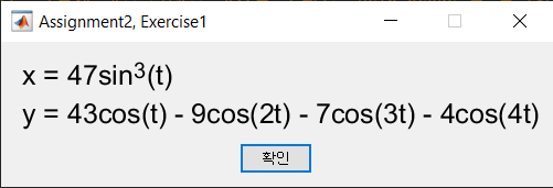
    >> MAS109_assign2_ex1(20219999)
   

   를 입력하여 다름과 같은 매개변수 함수 \(x,\, y\)를 얻을 수 있습니다.

   

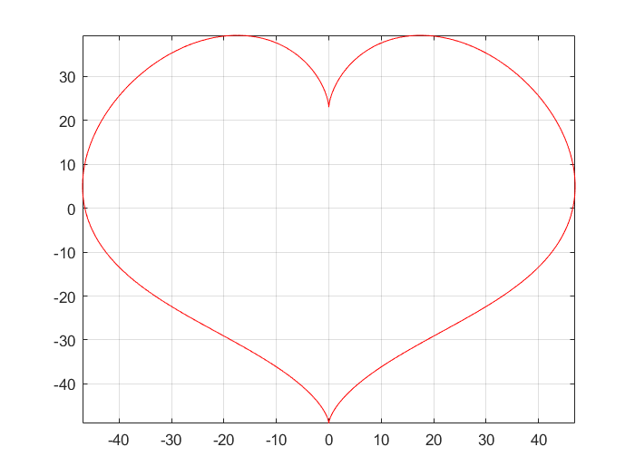
   매트랩 명령어 plot를 이용하여, 범위 \(-\pi \le t \le \pi\)에서 \((x, \, y)\)가 나태내는 그래프를 그릴 수 있습니다.

    t = -pi:0.01:pi;
    x = 47 * sin(t).^3;
    y = 43 * cos(t) - 9 * cos(2 * t) - 7 * cos(3 * t) - 4 * cos(4 * t);
   
    figure;
    plot(x, y, 'r');        % plot the graph of parametric x and y
    grid on; axis tight;
   

   MATLAB result

   

2. 학번이 20219999인 경우,

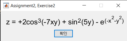
    >> MAS109_assign2_ex2(20219999)
   

   를 입력하여 다음과 같은 \(x,\,y\)에 대한 함수 \(z\)를 얻을 수 있습니다.

   

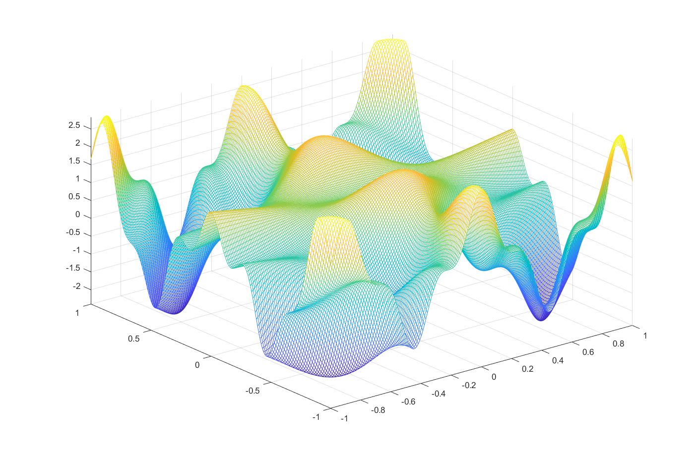
   매트랩 명령어 meshgrid와 mesh(또는 surf)를 이용하여, 범위 \(-1 \le x,\,y \le 1\)에서 \(z\)의 그래프를 그릴 수 있습니다.

   해답

    x = -1:0.01:1;              % set range of x, y as [-1, 1]
    y = x;
   
    [X, Y] = meshgrid(x, y);     % expand x, y to the rectangular grid
   
    Z = 2 * cos(-7 * X .* Y).^3 + sin(5 * Y).^2 - exp(-X.^2 - Y.^2);
   
    figure;
    mesh(X, Y, Z);              % plot the graph of parametric x and y
    grid on; axis tight;
   

   MATLAB result

   

0.2. 과제 3. 연습문제

1. 함수 \(f\)와 \(g\)가 다음과 같이 주어졌다고 해보겠습니다.

   \[\begin{align} f(x,\, y) &= e\sin(xy^2) + e\cos(x^2y),\\ g(z) &= \arctan(z). \end{align}\]

   앞선 문제들을 보고 \(f_{xy}(2,\,3)\)와

   \[\int_{-1}^{1} |g(z) - T_{g}^{9}(z)|^2 dz.\]

   의 값을 계산해보세요. 여기서 \(T_{g}^{9}(z)\)는, \(g(z)\)의 \(9\)차 항까지의 테일러 전개를 말합니다.

   Solution.

    syms x y z  % Declare symbolic variables x, y, z
   
    % Make functions f and g using the variables
    f = exp(sin(x * y^2)) + exp(-cos(x^2 * y));
    g = atan(z);
   
    fxy = diff(f, x, y);    % Calculate exact form of 'd^2f/dxdy'
    Vf = double(subs(fxy, [x, y], [2, -3]));  % find the value (d^2f/dxdy)(2, -3)
   
    % Compute Taylor expansion of g to the 9th order term
    T = taylor(g, z, 'Order', 10);
   
    h = abs(g - T)^2;   % The squared difference
   
    % Find the value of integration which is given in the assignment
    Vg = double(int(h, [-1, 1]));
   
    % Display
    fprintf('The value of f_xy(2,-3) is %f\n', Vf);
    fprintf('The L2 error between g and T on [-1, 1] is %f\n', Vg);
   

   MATLAB results

    The value of f_xy(2,-3) is -84.804965
    The L2 error between g and T on [-1, 1] is 0.000230
   

1. 들어가며

이번 내용은 짧지만 매우 중요합니다. 꼭 천천히 읽으면서 따라해보세요.

여러분은 무리수 \(\pi\)를 소수점 아래 몇번째 자리수까지 외울 수 있나요? 아마 많이 외울수는 없을거에요. 하지만, 테일러급수를 이용하면 \(\pi\)를 계산할 수 있어요. \(x\in[-1, 1]\)에서 \(\arctan\)의 테일러급수는 다음과 같습니다.

\[\arctan(x) = \sum_{n=0}^{\infty} {(-1)^{n}\frac{x^{(2n+1)}}{2n+1}} = x - \frac{x^3}{3} + \frac{x^5}{5} - \cdots, \quad -1 \le x \le 1.\]

또한, 우리는 \(\arctan(1)=\frac{\pi}{4}\)인 걸 알고있기 때문에,

\[\frac{\pi}{4} = 1 - \frac{1}{3} + \frac{1}{5} - \cdots,\]

이죠. 이것을 이용해서 직접 \(\pi\)를 계산해볼까요?

MATLAB codes

x = 1 - 1/3 + 1/5 - 1/7 + 1/9 - 1/11 + 1/13 - 1/15 + 1/17;
PI = 4 * x;
fprintf("PI = %.6f\n", PI);

MATLAB results

PI = 3.252366

어떤가요? 9번째 항까지 전개했지만, 우리가 예상한 \(\pi\)의 값 \(3.141592\dots\)와는 많이 다른 걸 알 수 있습니다. 만약 우리가 더 많은 항까지 전개하여 계산한다면, 더 정확한 결과를 얻을 수 있을거에요. 이런 경우에 직접 손으로 계산하는 건 한계가 있겠죠? 이럴때 for문과 while문을 이용해서 해결할 수 있습니다.

2. for 반복문

for 반복문은

for <변수> = <범위>
    <코드(변수)>
end

의 형태로 사용할 수 있습니다. <변수>가 <범위>의 처음부터 마지막까지 순차적으로 변화하는 동안, <변수>와 관련된 코드가 작동하는 것이지요. 간단한 예를 보겠습니다.

for i = [1, 2, 3, 4, 5, 6, 7, 8, 9, 10]
    fprintf("변수는 %d 입니다.\n", i);
end

변화하는 변수에 맞춰서 메시지가 출력됩니다. 만약 :구문을 이용한다면, 더 간단하게 바꿀 수 있습니다.

for i = 1:10
    fprintf("변수는 %d 입니다.\n", i);
end

그렇다면 이제 for문을 이용해 \(\pi\)의 값을 계산해봅시다.

MATLAB codes

pi_4 = 0;
for i = 0:10^5
    pi_4 = pi_4 + (-1)^i / (2 * i + 1);
end
PI = pi_4 * 4;
fprintf("PI = %.6f\n", PI)

MATLAB results

PI = 3.141603

무려 \(10^5\)째 항까지 계산했더니, 드디어 우리가 아는 \(\pi\)의 값과 비슷한 결과를 얻었습니다. 지금보니, 처음에 손으로 계산하려 한 것은 어림없는 시도였던 것이죠. 하지만, 우리는 아직도 만족할 수 없어요. 지금 얻은 결과조차도 실제 \(\pi\)와 비교하면 꽤 큰 오차가 있기 때문입니다.

3. while 반복문

for문을 이용해서 \(\pi\)의 값을 계산할때, 가장 어려운 것 중에 하나는 바로 <범위>를 정하는 것 입니다. 몇 번째 항까지 계산해야 원하는만큼 정확한 \(\pi\)의 값을 구해낼 수 있을지 모르기 때문이죠. 사실 조금만 분석해보면, \(n\)번째 항까지 계산했을 때 실제 \(\pi\)와의 오차가 어느정도인지 대략적으로 계산해낼 수 있습니다만, 그건 이 문서의 범위를 넘어서므로 다루지 않겠습니다. 대신 (아마도?)더 간단하게, while문을 이용해서 원하는 만큼 정확한 값을 구해내보죠. while문은,

while <조건>
    <코드>
end

와 같은 구조를 가집니다. 언뜻 보기엔 for문보다 더 간단해 보이는데요. 반복 횟수가 정해져있는 for문과는 달리, while문은 <조건>을 만족하는 동안은 계속해서 <코드>를 반복 실행 합니다. 예를들어,

i = 0;
while i < 10
    i = i + 1;
    fprintf("변수는 %d 입니다.\n", i);
end

와 같이 사용할 수 있죠. 다시 \(\pi\)를 구하는 문제로 돌아가 보겠습니다. 우리는 err변수를 정의해서, err가 원하는 값보다 작아져야 반복을 그만두는 코드를 작성할 것입니다. 이 과정에서, 우리가 알고있는 \(\pi\)의 값을 사용해서 err를 계산하겠습니다.

MATLAB codes

err = 999;                          % set initial error
pi_4 = 0;
pi_4_real = 3.1415926535 / 4;       % (approx) real value of pi / 4
i = 0;
while err >= 10^(-8)                % while `err` is not small enough
    pi_4 = pi_4 + (-1)^i / (2 * i + 1);
    err = abs(pi_4 - pi_4_real);
    i = i + 1;
end
PI = 4 * pi_4;
fprintf("PI = %.6f, order = %d\n", PI, i);

이제 \(\pi\)의 값을 소수점 7번째 자리까지 정확히 계산한 결과를 얻을 수 있습니다. 또한, 그러기까지 무려 24943984번째 항까지 전개를 해야한다는 것도 알 수 있네요. 이처럼, while문을 사용하면 for문으로는 해결하기 힘든 경우도 해결할 수 있습니다.

4. if 조건문

if 조건문의 핵심은 바로 ‘조건’이 무엇인가 하는 것인데요, 컴퓨터는 어떤 명제가 참인지 거짓인지를 숫자 0, 1로 판별합니다. 조건이 0이면 거짓, 1이면 참인 것이죠. 매트랩에서 이런 조건을 나타내는 방법은 (주로) ‘연산자’를 사용한 ‘조건식’을 사용하는 것입니다. 연산자의 종류는 대표적으로 ==, ~=(같음 연산자)와 <, <=, >, >=(관계 연산자)들이 있습니다. 매트랩 명령창에서,

1 == 1

을 입력하면 매트랩은 ‘참’이라는 뜻으로 1을 출력할 것입니다. 반대로

1 ~= 1

을 입력하면 ‘거짓’이라는 뜻으로 0을 출력하겠죠. 이처럼 두 수(뿐만아니라 두 행렬)간의 비교를 통한 조건식을 작성할 수 있습니다.
(C, C++, Java, Python 등 많은 언어들에서 두 수가 다름을 표현할 때 !=을 사용합니다. 하지만 매트랩의 경우는 ~=을 사용하니, 유의하세요.)

4.1. 간단한 if 조건문

if 조건문은 여러가지로 형태로 변형하여 사용할 수 있습니다. 그 중 가장 간단한 형태는 다음과 같습니다.

if <조건>
    <코드>
end

<조건>이 참(1)이면 <코드>를 실행하는 것이죠. 간단한 예를 보면,

x = 3;
if x < 5
    disp("x is less than 5.")
end

x가 숫자 5보다 작으면 알려주는 코드를 작성할 수 있습니다. 만약 첫 줄이 x=6과 같이 변한다면 아무것도 출력되지 않겠죠.

4.2. if-else 조건문

if-else 조건문은 두가지 경우의 수를 고려할 수 있는 조건문입니다. 다음과 같은 형태로 사용합니다.

if <조건>
    <코드1>
else
    <코드2>
end

만약 <조건>이 참이면 <코드1>을 실행하고, 그렇지 않으면 <코드2>를 실행하게 되는 것이죠. 예를들어 다음학기 수강신청때, 선형대수학개론이 재미있으면 선형대수학을 수강하고, 재미 없으면 선형대수학을 수강하지 않도록 결심하는 상황을 생각해 보면, 다음과 같이 나타낼 수 있을 것입니다.

MAS109 = input("Was MAS109 fun? Type 1 if it was.");
if MAS109 == 1
    disp("Let's go to take the MAS212");
else
    disp("Yes, it could be, I understand.");
end

변수 MAS109에 1이 저장되었을때와 그 외의 경우로 나누어서 출력문을 바꿀 수 있습니다.

4.3. if-elseif-else 조건문

여러가지 조건을 한번에 따져서 각 경우에 맞는 코드를 작동시킬 수 있습니다.

if <조건1>
    <코드1>
elseif <조건2>
    <코드2>
else
    <코드3>
end

이처럼 if-elseif-else조건문은, <조건1>이 참이면 <코드1>을, <조건1>이 거짓이소 <조건2>가 참이면 <코드2>를, <조건1>과 <조건2>가 모두 거짓이면 <코드3>을 실행하도록 작성할 수 있습니다.

5. continue와 break

1. continue

   if문을 사용하여 반복문 안의 코드를 선택적으로 실행할 수 있습니다. 예를들어, 1부터 100까지의 숫자들 중 홀수만 더하는 문제를 생각해보죠. 사실 이 문제는 if문을 사용하지 않아도 지난시간에 배운 for반복문을 사용하여 쉽게 해결할 수 있습니다.

    S = 0;
    for i = 1:2:100
        S = S + i;
    end
    fprintf("S = %d\n", S)
   

   다른방법으로도 해결할 수 있을까요? 반복문과 if문, continue를 사용하면 짝수는 건너뛰고 홀수만 반복적으로 더할 수 있습니다. 여기서 continue는 ‘이번 반복’을 건너뛰고 ‘다음 반복’으로 넘어갈 수 있게하는 역할을 합니다.
   (사실 이 방법이 더 비효율적이지만, continue함수를 직접 사용해보기 위해 보도록 하겠습니다.)

    S = 0;
    for i = 1:100
        if mod(i, 2) == 0
            continue        % skip this iteration
        end
        S = S + i;
    end
    fprintf("S = %d\n", S)
   

2. break

   break는 continue와는 조금 다르게 작동합니다. 반복문 안에서 break를 만나게되면, 현재 진행중인 반복문을 벗어나게 됩니다. 예를들어, 만약 우리가 while문의 조건을 1로 부여하면, 항상 참인 조건이기 때문에 while문은 무한히 반복될 것 입니다. 이렇게 무한히 반복되는 코드를 ‘무한 루프’라고 하는데, 실수로 무한 루프를 생성하게되면 강제로 코드 실행을 종료해야만 하는 상황이 생기게 됩니다. 이런 상황에서, 무한루프 안에 break를 삽입하게되면 조건과 상관없이 반복이 종료되고 while문의 end로 이동하게 됩니다.

    k = 0;
    while 1
        fprintf("Now k is %d\n", k);
        if k >= 10
            break
        end
        k = k + 1;
    end
   
    fprintf("Now the while-loop is broken\n")
   

6. function의 작성

매트랩의 편집기를 이용하면 스크립트 파일(*.m)을 작성할 수 있다는 건 이미 알고 있을겁니다. 스크립트 파일에 코드를 작성하여 저장해놓으면 원할때마다 불러와서 실행할 수 있습니다. 매트랩에서는 스크립트 파일을 단순 실행하는 것 뿐만 아니라 ‘함수’로 만들어서 입력값과 출력값을 가지도록 저장할 수 있습니다. 매트랩의 함수는 다음과 같은 형식을 가집니다.
(매트랩에서는 명령창에서 함수를 정의할 수 없습니다. 반드시 스크립트 파일로 작성한 뒤 저장하여 사용해야 합니다.)

function [<출력1>, <출력2>, ... ] = <함수이름>(<입력1>, <입력2>, ... )
    <코드>
end

함수는 여러개의 출력과 여러개의 입력을 가질 수 있습니다. 두 수를 입력받아 더하는 함수를 생각해보면:

% mySum.m
function aPb = mySum(a, b)
    aPb = a + b;
end

위 함수를 mySum.m이라는 이름으로 저장한 뒤, 명령창에 mySum(1, 3)을 입력하면 우리가 예상한 결과를 얻을 수 있습니다. 이 경우에는 출력되는 변수가 aPb하나밖에 없기때문에 []를 생략했지만, 여러개의 변수를 출력하는 함수의 경우는 반드시 []를 이용해야 합니다.

% mySumMul.m
function [aPb, aTb] = mySumMul(a, b)
    aPb = a + b;
    aTb = a * b;
end

이 함수역시 스크립트 파일로 저장한 뒤 명령창에서 mySumMul(3, 4)처럼 불러올 수 있습니다. 이 때, 따로 지정하지 않는다면 함수는 항상 첫번째 출력변수(aPb)만을 출력합니다. 만약 두 결과를 모두 출력받으려면, [x, y] = mySumMul(3, 4)와 같이 입력받을 변수들 각각에 대해 대응시켜주어야 합니다.

연습문제

1. 그래프를 그려서 다음 극좌표계의 교점의 개수를 찾으세요.

   \[\begin{cases} r = 1+\cos(k\theta)\\ r = \cos(k\theta)\\ \end{cases}, \qquad \text{where} \quad 0\le\theta\le 2\pi\]
   1. 매트랩의 hold명령어를 사용해서 하나의 극좌표계에 두개의 그래프를 동시에 나타내세요.
   2. 각각의 \(k = 1, 2, \cdots, 6\) 에 대하여 1번의 과정을 반복하세요. for문을 이용하여 쉽게 해결할 수 있습니다.
   3. 2번에서의 각 \(k\)에 대한 결과를 하나의 figure창에 나타내세요. \(2\times 3\) subplot들을 생성해서 해결하세요.

   각각 몇개의 교점을 가지고 있습니까?

2. 임의의 정사각행렬을 입력받아 행렬식을 출력하는 함수를 작성하세요.
   [힌트: 매트랩 함수는 자기 자신을 반복적으로 불러오는 형태로 작성될 수 있습니다. Co-factor 전개가 그 자체로 반복적인 형태를 갖는 걸 기억하세요.]

3. 주어진 행렬의 RREF를 찾는 함수 myRREF를 작성하세요.

   임의의 행렬에 대한 RREF를 찾는 함수를 작성하는건 다소 복잡합니다. 여기서는, 3가지 기본행연산 중 ‘두 행의 교환’을 사용하지 않고 가우스 소거법을 적용할 수 있는 행렬들에 대해서만 작동하는 함수를 작성하세요. 교과서 2.1의 연습문에 6 에서 이와같은 행렬을 발견할 수 있습니다.

4. 2번문제를 참고하여, ‘두 행의 교환’을 사용하지 않고 가우스 소거법을 적용할 수 있는 행렬들에 대하여 \(LU\)-분해를 하는 함수를 작성하세요.

---

Assignment 4

Assignment	4
Score	0
Submission	False

0. Solution to exercises

0.1. Exercises, assignment 2

1. Let ID number is 20219999. By entering the following codes in command window,

    >> MAS109_assign2_ex1(20219999)
   

   you can get parametric functions \(x,\, y\).

   

   Using the MATLAB command plot, you can plot the graph represented by \((x, \, y)\) in the range \(-\pi \le t \le \pi\).

    t = -pi:0.01:pi;
    x = 47 * sin(t).^3;
    y = 43 * cos(t) - 9 * cos(2 * t) - 7 * cos(3 * t) - 4 * cos(4 * t);
   
    figure;
    plot(x, y, 'r');        % plot the graph of parametric x and y
    grid on; axis tight;
   

   MATLAB result

   

2. Let ID number is 20219999. By entering the following codes in command window,

    >> MAS109_assign2_ex2(20219999)
   

   You can get the function \(z\) w.r.t. the variables \(x,\,y\) like the following.

   

   Using the MATLAB commands meshgrid and mesh (or surf), you can graph \(z\) in the range \(-1 \le x,\,y \le 1\).

    x = -1:0.01:1;              % set range of x, y as [-1, 1]
    y = x;
   
    [X, Y] = meshgrid(x, y);     % expand x, y to the rectangular grid
   
    Z = 2 * cos(-7 * X .* Y).^3 + sin(5 * Y).^2 - exp(-X.^2 - Y.^2);
   
    figure;
    mesh(X, Y, Z);              % plot the graph of parametric x and y
    grid on; axis tight;
   

   MATLAB result

   

0.2. Exercises, assignment 3

1. Let \(f\) and \(g\) be two functions given by

   \[\begin{align} f(x,\, y) &= e\sin(xy^2) + e\cos(x^2y),\\ g(z) &= \arctan(z). \end{align}\]

   Referring to the previous problems compute values of \(f_{xy}(2,\,3)\) and

   \[\int_{-1}^{1} |g(z) - T_{g}^{9}(z)|^2 dz,\]

   where the \(T_{g}^{9}(z)\) denotes \(9\)th order taylor expansion for \(g(z)\).

   Solution.

    syms x y z  % Declare symbolic variables x, y, z
   
    % Make functions f and g using the variables
    f = exp(sin(x * y^2)) + exp(-cos(x^2 * y));
    g = atan(z);
   
    fxy = diff(f, x, y);    % Calculate exact form of 'd^2f/dxdy'
    Vf = double(subs(fxy, [x, y], [2, -3]));  % find the value (d^2f/dxdy)(2, -3)
   
    % Compute Taylor expansion of g to the 9th order term
    T = taylor(g, z, 'Order', 10);
   
    h = abs(g - T)^2;   % The squared difference
   
    % Find the value of integration which is given in the assignment
    Vg = double(int(h, [-1, 1]));
   
    % Display
    fprintf('The value of f_xy(2,-3) is %f\n', Vf);
    fprintf('The L2 error between g and T on [-1, 1] is %f\n', Vg);
   

   MATLAB results

    The value of f_xy(2,-3) is -84.804965
    The L2 error between g and T on [-1, 1] is 0.000230
   

1. Intro

This is short, but very important. Please read carefully and follow along.

How many digits can you memorize the irrational number \(\pi\)? Maybe you can’t memorize that much. However, we can calculate \(\pi\) using the Taylor series. The Taylor series of \(\arctan\) where \(x\in[-1, 1]\) is:

\[\arctan(x) = \sum_{n=0}^{\infty} {(-1)^{n}\frac{x^{(2n+1)}}{2n+1}} = x - \frac{x^3}{3} + \frac{x^5}{5} - \cdots, \quad -1 \le x \le 1.\]

and since we know that \(\arctan(1)=\frac{\pi}{4}\),

\[\frac{\pi}{4} = 1 - \frac{1}{3} + \frac{1}{5} - \cdots,\]

Now, shall we use this to calculate \(\pi\)?

MATLAB codes

x = 1 - 1/3 + 1/5 - 1/7 + 1/9 - 1/11 + 1/13 - 1/15 + 1/17;
PI = 4 * x;
fprintf("PI = %.6f\n", PI);

MATLAB results

PI = 3.252366

We expanded to the 9th term, but we can see that it is very different from the value of \(\pi\) we expected \(3.141592\dots\). If we expand to more terms than 9th term, we will get more accurate result. But in that case, it is hard to calculate by hand coding. Thus we can use the for statement and the while statement.

2. for loop

In general, for loop looks like:

for <variable> = <range>
    <codes(variable)>
end

While <variable> changes sequentially from the beginning to the end of the <range>, the code related to <variable> is executed. Let’s look at a simple example.

for i = [1, 2, 3, 4, 5, 6, 7, 8, 9, 10]
    fprintf("The variable is %d.\n", i);
end

A message is displayed according to the changing variable i. If we use the : syntax, we can change it more simply.

for i = 1:10
    fprintf("The variable is %d.\n", i);
end

Then, let’s use the for statement to calculate the value of \(\pi\).

MATLAB codes

pi_4 = 0;
for i = 0:10^5
    pi_4 = pi_4 + (-1)^i / (2 * i + 1);
end
PI = pi_4 * 4;
fprintf("PI = %.6f\n", PI)

MATLAB results

PI = 3.141603

After calculating up to the \(10^5\)th term, we finally got a result similar to the value of \(\pi\) we know. Now we know that it was almost impossible to try to get accurate results by hand coding. But, we still can’t be satisfied. Because we want to calculate a more accurate value.

3. while loop

When calculating the value of \(\pi\) using the for statement, one of the most difficult things is determining the <range>. It’s because we don’t know if we need to calculate the number of terms to get the exact value of \(\pi\) as we want. In fact, if we analyze it a bit using math, we can roughly calculate how much the error is from the actual \(\pi\) when calculating to the \(n\)th term, but that is beyond the scope of this document, so I will not deal with it. Instead, we can use the while statement.

while <condition>
    <codes>
end

The while loop is looks like above. At first glance, it looks simpler than the for statement. Unlike the for statement, which has a fixed number of iterations, the while statement executes <code> repeatedly as long as the <condition> is satisfied.

i = 0;
while i < 10
    i = i + 1;
    fprintf("The variable is %d.\n", i);
end

You can use it as above. Let’s go back to the problem of finding \(\pi\). We’ll define a variable err, so we’ll write the code to stop loop if err is less than the desired value. In this process, we will calculate err using the value of \(\pi\) we know.

MATLAB codes

err = 999;                          % set initial error
pi_4 = 0;
pi_4_real = 3.1415926535 / 4;       % (approx) real value of pi / 4
i = 0;
while err >= 10^(-8)                % while `err` is not small enough
    pi_4 = pi_4 + (-1)^i / (2 * i + 1);
    err = abs(pi_4 - pi_4_real);
    i = i + 1;
end
PI = 4 * pi_4;
fprintf("PI = %.6f, order = %d\n", PI, i);

Now we can get the exact result of calculating the value of \(\pi\) to the 7th decimal place. In addition, it can be seen that in order to do so, it must be expanded to the 24943984th term. Like this, using the while statement can solve cases that are difficult to solve with the for statement.

4. if conditional statement

The key to the if conditional statement is what the ‘condition’ is, and the computer determines whether a certain proposition is true or false as the numbers 0 and 1. If the condition is 0, it is false, and if the condition is 1, it is true. The way to express these conditions in MATLAB is to use’conditional expressions’ using ‘operators’. Representative types of operators are ==, ~= (equality operator), <, <=, >, and >= (relational operator). In the MATLAB command window, if you enter

1 == 1

then MATLAB will output ‘1’, meaning’True’. Contrary, if you enter

1 ~= 1

then it will output ‘0’, meaning ‘false’. In this way, You can write a conditional expression by comparing two numbers like this.
(Many languages ​​such as C, C++, Java, and Python use != when expressing the difference between two numbers. However, in the case of MATLAB, ~= is used, so be careful.)

4.1. a simple if statement

if statement can be used in various forms. The simplest of them is:

if <condition>
    <code>
end

If <condition> is true (1), then <code> is executed. Looking at a simple example,

x = 3;
if x < 5
    disp("x is less than 5.")
end

You can write code that tells you if x is less than the number 5. If the first line changes like x=6, nothing will be printed.

4.2. if-else statement

if-else statement can take into account two cases. It is used in the following form.

if <condition>
    <code1>
else
    <code2>
end

If <condition> is true, <code1> is executed, otherwise <code2> is executed. For example, when enrolling for a course next semester, you could decide to take Linear Algebra if you are interested in the Introduction to Linear Algebra, and if it is not, you could not decide to take Linear Algebra. This can be written in the code:

MAS109 = input("Was MAS109 fun? Type 1 if it was.");
if MAS109 == 1
    disp("Let's go to take the MAS212");
else
    disp("Yes, it could be, I understand.");
end

4.3. if-elseif-else statement

You can run the code for each case by considering several conditions at once.

if <condition1>
    <code1>
elseif <condition2>
    <code2>
else
    <code3>
end

Here, <code1>is executed if <condition1> is true, <code2> is executed if <condition1> is false and <condition2> is true, and <code3>is executed if both <condition1> and <condition2> are false.

5. continueand break

1. continue

   You can use the if statement to selectively execute the code inside the loop. For example, consider the problem of adding only odd numbers from 1 to 100. In fact, this problem can be easily solved by using the for loop we learned last time without using the if statement.

    S = 0;
    for i = 1:2:100
        S = S + i;
    end
    fprintf("S = %d\n", S)
   

   Could it be solved in other ways? If you use a loop, if statement, and continue, even numbers can be skipped and only odd numbers can be added repeatedly. Here, continue allows you to skip the ‘this iteration’ and move on to the ‘next iteration’.
   (Actually, this method is more inefficient than the before, but let’s look at it to try the continue directly.)

    S = 0;
    for i = 1:100
        if mod(i, 2) == 0
            continue        % skip this iteration
        end
        S = S + i;
    end
    fprintf("S = %d\n", S)
   

2. break

   break works a little differently than continue. When it encounters break in the loop, it breaks the loop in progress. For example, if we give the condition of the while to 1, the while iterates infinitely because the condition is always true. Loop that repeats infinitely like this is called an ‘infinite loop’, and if you accidentally create an infinite loop, there is a situation where you have to forcibly terminate execution of the code. Anyway, in any loops, when a break is encountered, the loop ends regardless of the condition and moves to the end of the while statement.

    k = 0;
    while 1
        fprintf("Now k is %d\n", k);
        if k >= 10
            break
        end
        k = k + 1;
    end
   
    fprintf("Now the while-loop is broken\n")
   

6. function file

You probably already know that you can create script files (*.m) using MATLAB’s editor. If you write and save the code in the script file, you can load it and run it whenever you want. In MATLAB, you can not only simply execute a script file, but also make it a ‘function’ and save it to have input and output values. MATLAB functions have the following format: (You cannot define a function in the command window in Matlab. You must write it as a script file and save it for use.)

function [<output1>, <output2>, ... ] = <function name>(<input1>, <input2>, ... )
    <code>
end

Functions can have multiple outputs and inputs. Consider a function that takes two numbers and adds them:

% mySum.m
function aPb = mySum(a, b)
    aPb = a + b;
end

Save the above function as mySum.m and enter mySum(1, 3) in the command window to get the results we expected. In this case, because there is only one variable to be output, aPb, [] could be omitted, but in the case of a function that outputs multiple variables, you must use [].

% mySumMul.m
function [aPb, aTb] = mySumMul(a, b)
    aPb = a + b;
    aTb = a * b;
end

This function can also be saved as a script file and loaded as mySumMul(3, 4) in the command window. In this case, unless otherwise specified, the function always outputs only the first output variable (aPb). If you want to get both results, you need to match each of the variables to be assigned like [x, y] = mySumMul(3, 4).

Exercises

1. Find the number of intersections of the polar system

   \[\begin{cases} r = 1+\cos(k\theta)\\ r = \cos(k\theta)\\ \end{cases}, \qquad \text{where} \quad 0\le\theta\le 2\pi\]

   by drawing the polar curves in MATLAB.

   1. For a polar system, use the MATLAB command hold to graph two polar curves on the same set of axis.
   2. For \(k = 1, 2, \cdots, 6\), graph the polar curves of each polar systems. You may use for loop. Then, you will have 6 graphs because you have 6 polar systems.
   3. Display your resulting images with \(2 \times 3\) subplots in the same figure window.

   How many intersections are there in each system?

2. Write a function that takes an arbitrary square matrix and outputs the determinant.
   [Hint: Matlab functions can be written by calling itself, recurrently. Observe that the co-factor expansion has natural recursive form.]

3. Write a function myRREF that finds the RREF of a given matrix.

   Writing a function to find the RREF for an arbitrary matrix is ​​a bit complicated. Here, write a function that works only for matrices that can apply the Gaussian elimination method without using the third elementary row operation, the ‘row exchange’. You can find a matrix like this in exercise 6 in textbook 2.1.

4. Referring to problem 2, write a function that does \(LU\)-decomposition for matrices that can apply the Gaussian elimination method without using the third elementary row operation, the ‘row exchange’.