Assignment 5
과제 5
| 과제 | 5 |
|---|---|
| 점수 | 5 (+5) |
| 기한 | Oct 21, 11:59 PM |
| 제출 형식 | 매트랩 fig파일 (*.fig) |
| 제출 장소 | KLMS assignment 5 |
| 파일 | Download |
0. 연습문제 해설
-
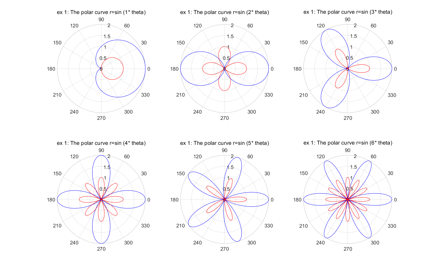
그래프를 그려서 다음 극좌표계의 교점의 개수를 찾으세요.
\[\begin{cases} r = 1+\cos(k\theta)\\ r = \cos(k\theta)\\ \end{cases}, \qquad \text{where} \quad 0\le\theta\le 2\pi\]% Create a linearly-spaced vector of the parameter domain theta theta = linspace(0, 2*pi, 200); figure(1); clf (1); % Open a figure window for k =1:6 r1 = 1 + cos(k * theta); % Calculate the values r1. r2=cos(k * theta); % Calculate the values r2. subplot(2, 3, k); polarplot(theta, r1, 'b'); % Draw the polar curve r hold on; polarplot(theta, r2, 'r'); title(sprintf('ex 1: The polar curve r=sin (%d* theta)', k)); endMATLAB results
-
임의의 정사각행렬을 입력받아 행렬식을 출력하는 함수를 작성하세요.
Solution.
function [D] = myDet (A) % A: input matrix , D: output % ( determinant of input matrix A) [m,n]= size (A); % the size of given input matrix A. D=0; % initialization of deteminant . if m~=n % if A is not a square matrix , % error message fprintf ('Error : given matrix is not a square matrix !\n'); else % othersize , if m == 2 % if input matrix A is 2x2 matrix , % compute the determinant using ad -bc. D = A(1, 1) * A(2, 2) - A(1, 2) * A(2, 1); else if m > 2 % if input matrix A is not 2x2 matrix , % In this for loop , we compute the determinant % of A by a cofactor expansion along the first % column of A using a recursive function call . for i = 1:m D = D + (-1)^(i+1) * A(i, 1) * myDet(A([1:i-1, i+1:m], 2:n)); end end end end end -
‘두 행의 교환’을 사용하지 않고 가우스 소거법을 적용할 수 있는 행렬들에 대하여 RREF를 찾는 함수
myRREF를 작성하세요.Solution.
function rref_A = rerowef (A) %- Finding Reduced Row Echelon Form without Row Interchanges -% [nrow , ncol ] = size (A); % The number of rows and columns of the matrix A. rref_A = A; % In order to initialize it , copy A to rref_A . % ---- Forward Phase ----% for i=1: nrow % Find the first nonzero entry of the ith row. for k=i: ncol if rref_A (i,k) ~= 0 break % Terminates the execution of the loop . end end rref_A (i ,:) = (1/ rref_A (i,k)) * rref_A (i ,:); % Normalize the pivot (i,k)-entry by 1 to the ith row. if i ~= nrow for j=(i+1) : nrow rref_A (j ,:) = ((- rref_A (j,k)) * rref_A (i ,:)) + rref_A (j, :); % Add minus (j,k)-entry times the ith row to the jth row. end end end % ---- Backward Phase ----% for i= nrow : -1:2 % Find the first nonzero entry of the ith row. for k=i: ncol if rref_A (i,k) ~= 0 break % Terminates the execution of the loop . end end for j=(i -1) : -1:1 rref_A (j ,:) = ((- rref_A (j,k)) * rref_A (i ,:)) + rref_A (j ,:); % Add minus (j,k)-entry times the ith row to the jth row. end end -
‘두 행의 교환’을 사용하지 않고 가우스 소거법을 적용할 수 있는 행렬들에 대하여 \(LU\)-분해를 하는 함수를 작성하세요.
Solution.
function [L, U] = ludecomp(A) % Find the LU - decomposition without using row interchanges. %- Finding the LU - decomposition without Row Interchanges -% [nrow , ncol] = size (A); % The number of rows and columns of the matrix A. U = A; L = eye(ncol); % Initialization of U and L. % ---- Forward Phase ----% for i = 1: nrow % Find the first nonzero entry of the ith row. for k=i:ncol if U(i,k) ~= 0 break % Terminates the execution of the loop. end end temp1 = U(i,k); % Save U(i,k) in temp. U(i, :) = (1/ temp1) * U(i, :); % Normalize the pivot (i,k)-entry by 1 to the ith row. L(i, i) = (1 / temp1)^(-1); % Place the reciprocal of the multiplier in that position in U. if i ~= nrow for j = (i+1):nrow temp2 = U(j, k);% Save U(j,k) in temp2. U(j, :) = ((-temp2) * U(i, :)) + U(j, :); % Add minus (j,k)-entry times the ith row to the jth row L(j,i) = -(-temp2); % Place the negative of the multiplier in that position U. end end end
1. 인덱싱
많은 사람들이 사용하는 언어인 Python에는 slicing이라는 개념이 있습니다. 특정 구조체의 일부를 불러오고 싶을때, 원하는 부분을 ‘긁어’올 수 있는 방법입니다. 매트랩의 행렬(과 벡터)에 대해서도, 똑같은 기능을 하는 indexing이 있습니다.
행렬 \(A\) 가 다음과 같이 주어졌다고 해보겠습니다.
A = [1, 2, 3, 4; 5, 6, 7, 8; 9, 10, 11, 12; 13, 14, 15, 16; 17, 18, 19, 20];
-
단일 요소 인덱싱
행렬의 특정 요소를 인덱싱할 수 있습니다. 예를들어, \(A\)의 3행 4열의 요소를 인덱싱하려면:
a34 = A(3, 4) -
벡터를 사용하여 여러 요소 인덱싱
같은 행 안에서 한번에 여러 요소를 인덱싱할 수 있습니다. 행렬 \(A\)의 4번째 열에서 4, 1, 3번째(순서에 유의) 행의 원소를 인덱싱하려면:
a4 = A([4, 1, 3], 4)또한, 여러 행과 열에 걸쳐있는 원하는 요소들을 한번에 인덱싱 할 수 있습니다. 행렬 \(A\)의 3번째와 2번째 행에서 각각 1, 2, 1번째 열들을 인덱싱하려면:
aa = A([3, 2], [1, 2, 1]) -
부분행렬 인덱싱
행렬 안에서 연속된 부분행렬을 추출할 수 있습니다. 행렬의 2 ~ 5행과 1 ~ 3열에 걸쳐있는 부분행렬을 인덱싱하려면:
(2:5는[2, 3, 4, 5]와 같으므로, 직접 벡터를 입력하여 인덱싱할 수도 있습니다.)B = A(2:5, 1:3)매트랩에서 인덱싱할 때, 행렬의 마지막 요소는
end로 대체하여 나타낼 수 있습니다. 즉, 위 구문은 아래와 같이 바꾸어 사용할 수 있습니다.B = A(2:end, 1:3)또한,
:구문을 잘 사용하면, 행(또는 열)을 거꾸로 세어서 인덱싱 할 수 있습니다.IB = A(end:-1:2, 1:3)행(또는 열)의 첫번째부터 마지막까지의 모든 요소를 선택하려면
:와 같이 처음과 끝을 생략하여 사용할 수 있습니다.C = A(:, :) % it is the same to APython에서도 똑같이
:와 같은 슬라이싱을 사용할 수 있습니다. 더불어서,3:과같이 한 쪽만 생략하여 처음과 끝을 나타낼 수 있죠. 하지만 매트랩에서는 Python과 달리 어느 한 방향만 생략하는 건 불가능하다는 걸 기억하세요. -
선형 인덱싱
명령창에
A(:)를 입력합니다. \(A\)는 분명 행렬이지만, 결과는 그렇지 않은 걸 알 수 있습니다. 이런 ‘선형 인덱싱’은 행렬의 요소들을 벡터형태로 다룰 수 있게 해줍니다. 예를들어, 행렬의 모든 요소의 합을 구할 때,sum(sum(A))나sum(A, 'a')대신sum(A(:))를 사용할 수 있겠죠. 익숙해진다면 매우 다양한 형태의 인덱싱을 구현할 수 있습니다. -
논리 인덱싱
명령창에
A > 5를 입력합니다. \(A\)의 요소들 중 5보다 큰 요소들이 있는 위치에1(True)값을 가지는 행렬이 반환됩니다. 우리는 이 논리행렬을 그래도 인덱싱에 사용할 수 있습니다.B_5 = A(A > 5)이런 경우, 결과값은 선형 인덱싱된 값으로 주어집니다. 응용하면, ‘\(A\)의 요소들 중, 5보다 큰 요소들만 -10으로 대체’하는 것과 같이 다소 복잡한 구현도 쉽게 할 수 있습니다.
A(A > 5) = -10
2. 이미지와 행렬
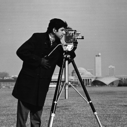
여러분은 (흑백)이미지를 하나의 행렬로 생각할 수 있다는 걸 알고있었나요? 컴퓨터에서 보는 디지털 이미지들은 각 픽셀(요소 위치)마다 하나의 화소값(행렬 값)을 가지는 행렬과 대응시켜 생각할 수 있습니다. 한번, 간단한 행렬을 만들고 imagesc함수를 사용해 행렬을 이미지와 같이 시각화해 보겠습니다.
A = reshape(1:20, 4, 5)';
figure;
imagesc(A); colormap gray;
또한, 임의의 이미지파일을 매트랩으로 불러와 행렬의 형태로 다룰 수 있습니다. 아래 이미지를 (jpg 또는 png)의 형태로 저장한 후, 매트랩의 imread명령어를 사용해 불러와 보세요. 이때 이미지 파일이 매트랩의 현재폴더에 위치해야 합니다. imshow명령어를 이용해서 시각화 하세요.
cman = imread('cameraman.png');
whos cman; % we can see that the `cman` is a matrix
figure;
imshow(cman); % and also `cman` is an image
연습문제
첨부된 파일들을 다운받으세요. 총 네개의 파일들, MAS109_assign5_ex1.p, MAS109_assign5_ex2.p, DATA.mat와 cameraman.png, 이 있습니다.
-
카메라맨 이미지를 매트랩에 불러오세요.
MAS109_assign5_ex1함수를, 본인의 학번을 입력값으로 실행한 후, 나타나는 정보를 확인하세요. 본인의 ‘Submatrix’항목에 나타난 ‘Rows’와 ‘Columns’를 참고하여, 카메라맨 이미지에서 해당하는 부분(부분행렬)만 figure 창에 표시하세요.imshow명령어 또는imagesc명령어를 사용해야할 수 있습니다. 생성한 figure 창을ex1_<studentID>.fig로 저장하세요.
(figure 창을 저장하는 방법은 이전 문서들에서 찾을 수 있습니다.) -
(추가 문제)
MAS109_assign5_ex2함수를, 본인의 학번을 입력값으로 실행한 후현재 폴더에 저장되는 이미지 파일을 확인하세요. 이미지 파일을 매트랩에 불러옵니다,imread명령어를 사용하세요. 그 후에, 다음 4개의 linear transformation을 순서대로 이미지에 적용하세요. 교재의 \(\mathrm{Figure}~6.2.4\)를 참고하세요. (이 문제는 반드시 제출할 필요는 없습니다. 다만, 올바르게 해결해서 제출한다면 다른 과제의 실수를 만회할 수 있는 점수 5점을 획득할 수 있습니다.)-
Expansion (or compression) in the \(y\)-direction with factor \(k_1\).
-
Contraction (or dilation) with factor \(k_2\).
-
Shear in the \(x\)-direction with factor \(k_3\).
-
Rotation about the origin through an angle \(k_4\).
imshow명령어는 주어진 grid 밖의 값은 표시하지 못합니다. 이미지가 하나의 행렬이라는 걸 생각하면서,surface등의 함수를 이용해 표시해보세요. -
제출
연습문제의 1번에서 저장한 ex1_<studentID>.fig를 KLMS의 지정된 장소에 제출하세요. 제출기한과 점수를 확인하시기 바랍니다.
Assignment 5
| Assignment | 5 |
|---|---|
| Score | 5 (+5) |
| Due date | Oct 21, 11:59 PM |
| Submission form | A MATLAB figure file (*.fig) |
| Where to submit | KLMS assignment 5 |
| Files | Download |
0. Solution to exercises
-
Find the number of intersections of the polar system
\[\begin{cases} r = 1+\cos(k\theta)\\ r = \cos(k\theta)\\ \end{cases}, \qquad \text{where} \quad 0\le\theta\le 2\pi\]Solution
 % Create a linearly-spaced vector of the parameter domain theta
 theta = linspace(0, 2*pi, 200);

 figure(1); clf (1);             % Open a figure window
 for k =1:6
     r1 = 1 + cos(k * theta);    % Calculate the values r1.
     r2=cos(k * theta);          % Calculate the values r2.
     subplot(2, 3, k);
     polarplot(theta, r1, 'b');  % Draw the polar curve r

     hold on;
     polarplot(theta, r2, 'r');
     title(sprintf('ex 1: The polar curve r=sin (%d* theta)', k));
 end
MATLAB results
-
Write a function that takes an arbitrary square matrix and outputs the determinant.
Solution.
function [D] = myDet (A) % A: input matrix , D: output % ( determinant of input matrix A) [m,n]= size (A); % the size of given input matrix A. D=0; % initialization of deteminant . if m~=n % if A is not a square matrix , % error message fprintf ('Error : given matrix is not a square matrix !\n'); else % othersize , if m==2 % if input matrix A is 2x2 matrix , % compute the determinant using ad -bc. D=A(1 ,1)*A(2 ,2) -A(1 ,2)*A(2 ,1); else if m >2 % if input matrix A is not 2x2 matrix , % In this for loop , we compute the determinant % of A by a cofactor expansion along the first % column of A using a recursive function call . for i=1: m D=D+( -1) ^(i+1)*A(i ,1)* myDet (A ([1:i -1, i+1:m], 2:n)); end end end end end -
Write a function
myRREFthat finds the RREF of matrices to which we can apply the Gaussian elimination method without using the third elementary row operation, the ‘row exchange’.Solution.
function rref_A = rerowef (A) %- Finding Reduced Row Echelon Form without Row Interchanges -% [nrow , ncol ] = size (A); % The number of rows and columns of the matrix A. rref_A = A; % In order to initialize it , copy A to rref_A . % ---- Forward Phase ----% for i=1: nrow % Find the first nonzero entry of the ith row. for k=i: ncol if rref_A (i,k) ~= 0 break % Terminates the execution of the loop . end end rref_A (i ,:) = (1/ rref_A (i,k)) * rref_A (i ,:); % Normalize the pivot (i,k)-entry by 1 to the ith row. if i ~= nrow for j=(i+1) : nrow rref_A (j ,:) = ((- rref_A (j,k)) * rref_A (i ,:)) + rref_A (j, :); % Add minus (j,k)-entry times the ith row to the jth row. end end end % ---- Backward Phase ----% for i= nrow : -1:2 % Find the first nonzero entry of the ith row. for k=i: ncol if rref_A (i,k) ~= 0 break % Terminates the execution of the loop . end end for j=(i -1) : -1:1 rref_A (j ,:) = ((- rref_A (j,k)) * rref_A (i ,:)) + rref_A (j ,:); % Add minus (j,k)-entry times the ith row to the jth row. end end -
Write a function that does \(LU\)-decomposition for matrices that can apply the Gaussian elimination method without using the third elementary row operation, the ‘row exchange’.
Solution.
function [L, U] = ludecomp(A)
% Find the LU - decomposition without using row interchanges.

%- Finding the LU - decomposition without Row Interchanges -%
[nrow , ncol] = size (A);   % The number of rows and columns of the matrix A.
U = A; L = eye(ncol);       % Initialization of U and L.

% ---- Forward Phase ----%
for i = 1: nrow
    % Find the first nonzero entry of the ith row.
    for k=i:ncol
        if U(i,k) ~= 0
            break           % Terminates the execution of the loop.
        end
    end

    temp1 = U(i,k);         % Save U(i,k) in temp.
    U(i, :) = (1/ temp1) * U(i, :);
    % Normalize the pivot (i,k)-entry by 1 to the ith row.
    L(i, i) = (1 / temp1)^(-1);
    % Place the reciprocal of the multiplier in that position in U.

    if i ~= nrow
        for j = (i+1):nrow
            temp2 = U(j, k);% Save U(j,k) in temp2.
            U(j, :) = ((-temp2) * U(i, :)) + U(j, :);
            % Add minus (j,k)-entry times the ith row to the jth row
            L(j,i) = -(-temp2);
            % Place the negative of the multiplier in that position U.
        end
    end
end
1. Indexing
Python, a language used by many people, has a concept called slicing. When you want to load a part of a specific structure, it is a way to ‘scrape’ the desired part. For MATLAB matrices(and vectors), there is indexing that does the same thing.
Let a matrix \(A\) be given:
A = [1, 2, 3, 4; 5, 6, 7, 8; 9, 10, 11, 12; 13, 14, 15, 16; 17, 18, 19, 20];
-
Indexing with a Single Index
We can index a specific element of the matrix. For example, to index the element in 3rd row and 4th column of \(A\):
a34 = A(3, 4) -
Indexing multiple elements using vectors
Multiple elements can be indexed at once within the same row(or column). To index the elements of the 4th, 1st, and 3rd rows(in that order) of the 4th column of the matrix \(A\):
a4 = A([4, 1, 3], 4)Also, you can index the elements you want across multiple rows and columns at once. To index the 1st, 2nd, and 1st columns of the 3rd and 2nd rows of matrix \(A\), respectively:
aa = A([3, 2], [1, 2, 1]) -
Submatrix indexing
We can extract contiguous submatrices within a matrix. To index submatrices spanning 2-5 rows and 1-3 columns of a matrix:
(Since2:5is the same as[2, 3, 4, 5], you can also directly input vectors for indexing.)B = A(2:5, 1:3)When indexing in MATLAB, the last element of the matrix can be represented by substituting
end. In other words, the above syntax can be used interchangeably as shown below.B = A(2:end, 1:3)Also, if you use the
:syntax well, you can index rows (or columns) by counting them backwards.IB = A(end:-1:2, 1:3)To select all elements from the first to the last of a row (or column), you can omit the beginning and end, such as
:.C = A(:, :) % it is the same to AIn the Python, you can also use slicing syntax
:. In addition, the beginning and end can be omitted only one side, such as3:. However, remember that in MATLAB, unlike Python, it is impossible to omit only one side. -
Linear indexing
Enter
A(:)in the command window. You can see that \(A\) is definitely a matrix, but the result is not. This ‘linear indexing’ allows the elements of a matrix to be manipulated in vector form. For example, to sum all the elements of a matrix, you could usesum(A(:))instead ofsum(sum(A))orsum(A,'a'). Once you get used to it, you can implement many variery forms of indexing. -
Logial indexing
Enter
A> 5in the command window. A matrix with a value of1(True) is returned where there are elements greater than 5 among the elements of \(A\). We can also use this logical matrix for indexing.B_5 = A(A > 5)In this case, the result is given as a form of linearly indexing. If applied, it is easy to implement rather complex implementations such as ‘replace only elements larger than 5 among the elements of \(A\) with -10’.
A(A > 5) = -10
2. Image and matrix
Did you know that we can think of a (grayscale) image as a matrix? Digital images viewed on a computer can be thought of as matching a matrix with one pixel value (matrix value) for each pixel (element position). First, let’s create a simple matrix and use the imagesc function to visualize the matrix like an image.
A = reshape(1:20, 4, 5)';
figure;
imagesc(A); colormap gray;
Also, arbitrary image files can be imported into MATLAB and handled in the form of a matrix. Save the image below in the form of (jpg or png), and then load it using MATLAB’s imread command. Note that the image file must be located in the Current Folder of MATLAB. Visualize using the imshow command.
cman = imread('cameraman.png');
whos cman;      % we can see that the `cman` is a matrix

figure;
imshow(cman);   % and also `cman` is an image
Exercises
Download the attached files. There are totally four files, MAS109_assign5_ex1.p, MAS109_assign5_ex2.p, DATA.mat and cameraman.png.
-
Load the cameraman image to MATLAB. Execute the
MAS109_assign5_ex1function with your student ID number as an input and check the information displayed. Refer to ‘Rows’ and ‘Columns’, and display only the corresponding part (submatrix) in the cameraman image in a figure window. You may need to use theimshowcommand or theimagesccommand. Save the created figure window asex1_<studentID>.fig.
(If you do not know how to save the figure window, back to the previous documents.) -
(Supplementary problem) Execute the
MAS109_assign5_ex2function with your student number as an input value and check the image file saved in thecurrent folder. Load the image file into MATLAB, use theimreadcommand. After that, apply the following 4 linear transformations to the image in order. Please refer to \(\mathrm{Figure}~6.2.4\) in the textbook. (You are not required to submit this problem. However, if you solve it correctly and submit it, you can get extra 5 points to make up for mistakes in other assignments.)-
Expansion (or compression) in the \(y\)-direction with factor \(k_1\).
-
Contraction (or dilation) with factor \(k_2\).
-
Shear in the \(x\)-direction with factor \(k_3\).
-
Rotation about the origin through an angle \(k_4\).
The
imshowcommand does not display values outside the given grid. By considering that image is a matrix, display it using a function such assurface. -
Submission
Submit the ex1_<studentID>.fig file saved in exercises 1 to the designated location in KLMS. Please check the submission deadline and score.
Leave a comment