Assignment 6

October 29, 2021 17 minute read

과제	6
점수	0 (+ 5)
기한	Nov 11, 11:59 PM
제출 형식	한 개의 매트랩 함수 파일 (*.m)
제출 장소	KLMS assignment 6

“디버깅이란, 컴퓨터 프로그램 개발 단계 중에 발생하는 시스템의 논리적인 오류나 비정상적 연산(버그)을 찾아내고 그 원인을 밝히고 수정하는 작업 과정을 뜻한다.”

위키백과의 ‘디버그’항목에서 말하는 디버깅의 정의입니다. 우리가 어떤 목적을 가지고 코드를 작성했을때, 작성된 코드가 한 번에 모든 기능을 올바르게 수행하는 경우는 많지 않습니다. 대부분의 경우는, 작성하면서 고려하지 못한 문제점들이 나타나기 마련이죠. 이럴 때 코드의 잘못된 부분을 찾아내고, 수정하는 작업을 디버깅이라고 합니다. 매트랩은 디버깅을 편하게 해주는 여러 기능을 가지고 있는데요, 그 중 몇 가지를 살펴보겠습니다.

0. 연습문제 해설

첨부된 파일들을 다운받으세요. 총 네개의 파일들, MAS109_assign5_ex1.p, MAS109_assign5_ex2.p, DATA.mat와 cameraman.png, 이 있습니다.

카메라맨 이미지를 매트랩에 불러오세요. MAS109_assign5_ex1함수를, 본인의 학번을 입력값으로 실행한 후, 나타나는 정보를 확인하세요. 본인의 ‘Submatrix’항목에 나타난 ‘Rows’와 ‘Columns’를 참고하여, 카메라맨 이미지에서 해당하는 부분(부분행렬)만 figure 창에 표시하세요. imshow명령어 또는 imagesc명령어를 사용해야할 수 있습니다. 생성한 figure 창을 ex1_<studentID>.fig로 저장하세요.
(figure 창을 저장하는 방법은 이전 문서들에서 찾을 수 있습니다.)

Solution.

사용자의 학번이 20219999라고 하면,
```
 >> MAS109_assign5_ex1(20219999);
```
를 입력하여 다음과 같은 결과를 얻을 수 있습니다.

또한, 카메라맨 이미지를 불러와 cman변수에 저장합니다.
```
 cman = imread("cameraman.png"); % make sure the png file is in the `current folder`.
```
```
 ex1 = cman(83:241, 64:221);     % extract an appropriate submatrix `ex1`.
 figure;
 imshow(ex1);
 savefig('ex1_20219999.fig');
```
MATLAB result.
(추가 문제) MAS109_assign5_ex2함수를, 본인의 학번을 입력값으로 실행한 후 현재 폴더에 저장되는 이미지 파일을 확인하세요. 이미지 파일을 매트랩에 불러옵니다, imread명령어를 사용하세요. 그 후에, 다음 4개의 linear transformation을 순서대로 이미지에 적용하세요. 교재의 \(\mathrm{Figure}~6.2.4\)를 참고하세요. (이 문제는 반드시 제출할 필요는 없습니다. 다만, 올바르게 해결해서 제출한다면 다른 과제의 실수를 만회할 수 있는 점수 5점을 획득할 수 있습니다.)
1. Expansion (or compression) in the \(y\)-direction with factor \(k_1\).
2. Contraction (or dilation) with factor \(k_2\).
3. Shear in the \(x\)-direction with factor \(k_3\).
4. Rotation about the origin through an angle \(k_4\).
imshow명령어는 주어진 grid 밖의 값은 표시하지 못합니다. 이미지가 하나의 행렬이라는 걸 생각하면서, surface등의 함수를 이용해 표시해보세요.

Solution.
- 문제에서 정확한 셋팅을 제시하지 않았기 때문에, 이 문제를 해결하기위해 쓸 수 있는 방법은 한 가지가 아닐 수 있습니다. 또한, 제시한 것을 잘 해결했다고 하더라고, 사용한 방법에 따라서 결과물이 다르게 보일 수 있습니다.
사용자의 학번이 20219999라고 하면,
```
 >> MAS109_assign5_ex2(20219999);
```
를 입력하여 다음과 같은 결과를 얻을 수 있으며, 현재 폴더에 For_20219999.png가 저장되는 걸 볼 수 있습니다.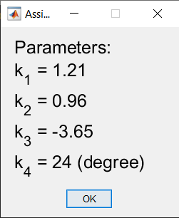

\(k_1,\,k_2,\,k_3,\,k_4\)에 해당하는 linear transformation의 representative matrix를 각각 \(T_1,\,T_2,\,T_3,\,T_4\)라고 하면, 각각을 순서대로 적용해 나가는 과정은 다음과 같습니다.
```
 % load image
 img = imread('For_20219999.png');
 [m, n] = size(img);
 [Y, X] = meshgrid(0:n-1, 0:m-1);

 % given parameters
 k1 = 1.21;
 k2 = 0.96;
 k3 = -3.65;
 k4 = 24;

 % representative matrices for each parameter
 % for simplicity, we can use 'cell' which is a
 % structure independent of data type.
 T{1} = [1, 0; 0, k1];
 T{2} = [k2, 0; 0, k2];
 T{3} = [1, k3; 0, 1];
 T{4} = [cosd(24), -sind(24); sind(24), cosd(24)];

 % for numerical computations
 flatX = reshape(X, 1, []);
 flatY = reshape(Y, 1, []);
 flatXY = [flatY; flatX];

 % applying each transformation
 for i = 1:4
     TXY{i} = T{i} * flatXY;
     TY{i} = reshape(TXY{i}(1, :), m, []);
     TX{i} = reshape(TXY{i}(2, :), m, []);
 end

 % visualization
 figure();
 subplot(2, 3, [1, 4]);
 surface(Y, X, img(end:-1:1, :), 'LineStyle', 'none');
 colormap gray; axis tight;
 subplst = [2, 3, 5, 6];
 for i = 1:4
     subplot(2, 3, subplst(i));
     surface(TY{i}, TX{i}, img(end:-1:1, :), 'LineStyle', 'none');
     colormap gray; axis tight;
 end
```
MATLAB results.

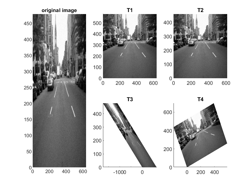
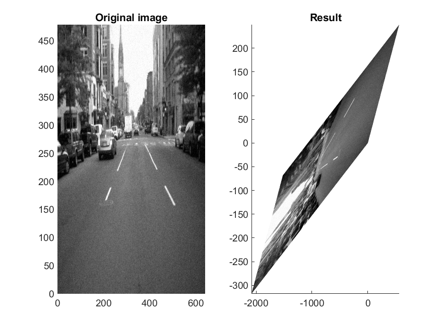
여기서, 이미지의 \(x\), \(y\) 축으로의 방향이 생각과 다르게 나타난다고 느낄 수 있습니다. 이미지를 좌표축에 올려놓는 방법은 여러가지로 정의될 수 있기 때문에, 이 부분은 크게 신경쓰기 않아도 됩니다. 다만, 내가 정한 좌표축에서 이미지가 예상한대로 잘 변형되고 있는지는 주의깊게 살펴봐야 합니다. 다음으로, 문제에서 제시한 것 처럼 모든 선형변환을 순서대로 적용한 결과는 다음과 같습니다.
```
 % load image
 img = imread('For_20219999.png');
 [m, n] = size(img);
 [Y, X] = meshgrid(0:n-1, 0:m-1);

 % given parameters
 k1 = 1.21;
 k2 = 0.96;
 k3 = -3.65;
 k4 = 24;

 % representative matrices for each parameter
 T1 = [1, 0; 0, k1];
 T2 = [k2, 0; 0, k2];
 T3 = [1, k3; 0, 1];
 T4 = [cosd(24), -sind(24); sind(24), cosd(24)];

 % for numerical computations
 flatX = reshape(X, 1, []);
 flatY = reshape(Y, 1, []);
 flatXY = [flatY; flatX];

 % applying the transformation
 TXY = T4*T3*T2*T1*flatXY;
 TY = reshape(TXY(1, :), m, []);
 TX = reshape(TXY(2, :), m, []);

 % visualization
 figure();
 subplot(1, 2, 1);
 surface(Y, X, img(end:-1:1, :), 'LineStyle', 'none');
 colormap gray; axis tight;
 title('Original image');
 subplot(1, 2, 2);
 surface(TY, TX, img(end:-1:1, :), 'LineStyle', 'none');
 colormap gray; axis tight;
 title('Result');
```
MATLAB results.

1. 중단점

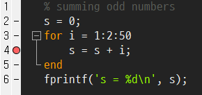
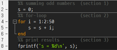
매트랩의 에디터는 자체적으로 중단점을 설정할 수 있는 기능이 있습니다. 다음과 같은 간단한 스크립트 파일을 작성한 뒤,

% summing odd numbers
s = 0;
for i = 1:2:50
    s = s + i;
end

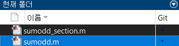
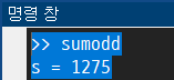
상단 편집기 탭의 실행 버튼을 누르거나, 키보드의 F5 키를 눌러서 현재 스크립트를 실행할 수 있습니다.

>> sumodd
s = 625

이제, 4번째 줄의 왼쪽 -표시를 누르거나, 해당 줄에 커서를 두고 F12를 눌러서 중단점을 설정해보세요.

result

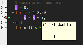
이 상태에서 코드를 실행시키면, 처음 만난 4번째 줄에서 더 이상 진행하지 않고 멈춰있는 걸 알 수 있습니다. 단순히 멈춘 것 뿐만 아니라, 이 상태에서 명령창과 작업공간을 활용하여 현재 멈춰있는 지점에서의 변수들을 확인할 수 있어요. 명령창의 K>>는 현재 코드가 중단점에서 멈춰있다는 뜻입니다.

K>> [i, s]

ans =

     1     0

혹은, 마우스 포인터를 변수 위에 올려서 해당 변수의 정보를 확인할 수도 있습니다.

result

상단의 계속 버튼을 누르거나 F5 키를 눌러서 멈춰있는 코드를 다시 실행할 수 있습니다. 코드를 다시 실행해도 화살표가 잠깐 깜빡일 뿐, 달라진 것 없이 비슷해 보입니다. 하지만, 실제로는 for문의 다음 단계까지 진행한 뒤에 다시 4번째 줄에서 멈추었다는 걸 확인할 수 있습니다.

[i, s]

ans =

     3     1

코드를 끝까지 실행하고 싶으면, 중단점을 해제하고 F5를 눌러서 재개할 수 있습니다. 혹은, 중단된 코드를 실행하지 않고 멈추려면, 상단의 디버그 중지 버튼이나 shift+F5를 이용할 수 있습니다.

2. 섹션 설정

우리는 %는 매트랩에서 특정 문장을 주석처리할 수 있습니다. 만약 %%와같이 두번 연속으로 사용하면, 해당 줄이 주석 처리되는 것 뿐만 아니라, 그 이후의 줄이 새로운 섹션으로 설정됩니다. 섹션의 범위는 새로운 섹션을 만들어서 설정할 수 있습니다.

result

특정 섹션에 속한 코드만 실행하거나, 다음 섹션으로 빠르게 넘어갈 수 있습니다.

섹션 별 실행

상단 편집기 탭의 섹션 실행을 누르거나, ctrl+enter를 누르면 현재 커서가 위치한 섹션만 실행할 수 있습니다.
섹션 진행

상단 편집기 탭의 진행을 누르거나, ctrl+↓를 누르면 현재 커서가 위치한 섹션에서 다음 섹션의 가장 처음으로 커서를 옮길 수 있습니다.
섹션 실행 및 진행

상단 편집기 탭의 실행 및 진행을 누르거나, ctrl+shift+enter를 누르면 현재 커서가 위치한 섹션을 실행하고, 다음 섹션으로 진행할 수 있습니다.

3. 선택 영역 실행

섹션을 따로 지정하지 않나도, 선택한 영역을 바로 명령창에서 실행할 수 있습니다. 실행하고자 하는 영역을 선택한 후, F9를 눌러서 실행하세요. 코드의 일부 또는 전부, 현재 폴더에 있는 파일 또는 이전 실행한 기록의 일부 등 어떤 것이든지 바로 실행할 수 있습니다.

선택 영역

result

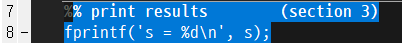
F9 결과

 >> % print results        (section 3)
 fprintf('s = %d\n', s);
 s = 0

선택 영역

F9 결과
```
 >> sumodd
 s = 625
```

선택 영역

result

F9 결과

 >> sumodd
 s = 625
 s = 625

 s =

 625

연습문제

과제 4의 연습문제에서, 우리는 3가지 기본행연산 중 ‘두 행의 교환’을 사용하지 않고 가우스-조르단 소거법을 적용할 수 있는 행렬들에 대해서만 작동하는 rref 함수를 작성하였습니다. 여기서는 임의의 행렬에 대해 적용할 수 있는 my_rref.m함수를 작성하려 합니다. 아래에 주어진 가이드 코드의 빈칸을 채워서 코드를 완성하세요. (이 문제는 반드시 제출할 필요는 없습니다. 다만, 올바르게 해결해서 제출한다면 다른 과제의 실수를 만회할 수 있는 점수 5점을 획득할 수 있습니다.)

function rref_A = my_rref(A)
% Find the reduced row echelon form of A
% by performing Gauss-Jordan elimination with partial pivoting.

[m, n] = size(A);
rref_A = A;             % Initialization of rref_A as A.

% Forward phase with row interchanges.
rowIdx = 1;             % Count row.
for colIdx = 1:n
    % Find element to interchange two rows.
    [maxEntry, maxIdx] = max(abs(rref_A(rowIdx:m, colIdx)));
    
    if ---BLANK---      % If this column is a non-zero vector,
                        % then store index of pivot column.
                        % This part is more complicated than it looks.
                        % You may need to consider the 'round-off error'
        pivotCols(rowIdx) = colIdx;
        % Interchanging two rows.
        ---BLANK---;
        % Normalizing current row.
        rref_A(rowIdx, :) = ---BLANK---;
        % Successive row operation.
        for r = ---BLANK---
            rref_A(r, :) = rref_A(r, :) - rref_A(r, colIdx) * rref_A(rowIdx, :);
        end
        rowIdx = rowIdx + 1;    % Move onto the next row.
    end
    if rowIdx > m      	% If it was finished, stop.
        break
    end
end

% Backward phase.
preLding1Row = 0;
for pc = ---BLANK---    % Find only the pivot columns.
    
    % This is looking for the index of row in which leading 1 is appeared .
    for lding1Row = m - preLding1Row:-1:1
        preLding1Row = ---BLANK---;
        if rref_A(lding1Row, pc) >= ---BLANK---
            break       % here, you should focus on the value of `lding1Row`.
        end
    end
    for r = (lding1Row - 1):-1:1
        % Add 'minus (r, pivotCol)-entry times the ith row' to the kth row.
        rref_A(r, :) = ---BLANK---;
    end
end
end

제출

연습문제에서 완성한 my_rref.m파일을 KLMS의 지정된 장소에 제출하세요. 제출기한과 점수를 확인하시기 바랍니다. (이 문제는 반드시 제출할 필요는 없습니다. 다만, 올바르게 해결해서 제출한다면 다른 과제의 실수를 만회할 수 있는 점수 5점을 획득할 수 있습니다.)

채점 기준

임의로 생성된 여러개의 행렬들에 대해 시험한 뒤 채점될 것 입니다. 제출하기 전에, 되도록 많은 경우를 시험해보세요.
제출된 파일은 반드시 매트랩 함수로서 동작해야 합니다. 다시 말하면,
```
 >> R = my_rref(A);
```
위 명령어를 실행했을 때 R은 A의 rref가 되어야 합니다.
학생들끼리 혹은 인터넷에 있는 코드를 ‘참고’ 하는 건 아주 좋습니다. 다만, 참고한 뒤에 완전히 똑같은 코드를 제출하지 마세요. 이 번 과제가 0점이 되는 것 보다 더 큰 불이익이 있을 수 있습니다.

Assignment 6

Assignment	6
Score	0 (+ 5)
Due date	Nov 11, 11:59 PM
Submission form	One MATLAB function file (*.m)
Where to submit	KLMS assignment 6

“Debugging is the process of finding and resolving bugs (defects or problems that prevent correct operation) within computer programs, software, or systems.”

This is the definition of debugging, as referred to in Wikipedia’s ‘Debugging’ topic. When we write code for a certain purpose, it is unlikely that the code will perform all tasks correctly at once. In most cases, there are problems that you didn’t consider while writing. In this case, we should finding and correcting the wrong part of the code and that is called debugging. MATLAB has several tools that make debugging easier, let’s look at a few of them.

0. Solution for assignment 5

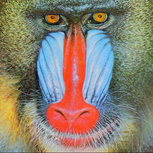
Download the attached files. There are totally four files, MAS109_assign5_ex1.p, MAS109_assign5_ex2.p, DATA.mat and cameraman.png.

Load the cameraman image to MATLAB. Execute the MAS109_assign5_ex1 function with your student ID number as an input and check the information displayed. Refer to ‘Rows’ and ‘Columns’, and display only the corresponding part (submatrix) in the cameraman image in a figure window. You may need to use the imshow command or the imagesc command. Save the created figure window as ex1_<studentID>.fig.
(If you do not know how to save the figure window, back to the previous documents.)

Solution.

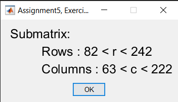
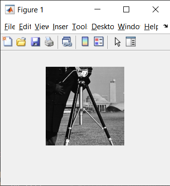
If the user’s student ID is 20219999, by entering:
```
 >> MAS109_assign5_ex1(20219999);
```
you can get the following result.

And also, load the cameraman image and store the variable cman.
```
 cman = imread("cameraman.png"); % make sure the png file is in the `current folder`.
```
```
 ex1 = cman(83:241, 64:221);     % extract an appropriate submatrix `ex1`.
 figure;
 imshow(ex1);
 savefig('ex1_20219999.fig');
```
MATLAB result.

(Supplementary problem) Execute the MAS109_assign5_ex2 function with your student number as an input value and check the image file saved in the current folder. Load the image file into MATLAB, use the imread command. After that, apply the following 4 linear transformations to the image in order. Please refer to \(\mathrm{Figure}~6.2.4\) in the textbook. (You are not required to submit this problem. However, if you solve it correctly and submit it, you can get extra 5 points to make up for mistakes in other assignments.)

Expansion (or compression) in the \(y\)-direction with factor \(k_1\).
Contraction (or dilation) with factor \(k_2\).
Shear in the \(x\)-direction with factor \(k_3\).
Rotation about the origin through an angle \(k_4\).

The imshow command does not display values outside the given grid. By considering that image is a matrix, display it using a function such as surface.

Solution.

Since the problem did not provide the exact settings, there may be several available methods to solve this problem. Also, even if the problem is well solved, the result may look different depending on the method used.

If the user’s student ID is 20219999, by entering

 >> MAS109_assign5_ex2(20219999);

you can get the following result and an image file For_20219999.png

result

If the representative matrix of the linear transformation corresponding to \(k_1,\,k_2,\,k_3,\,k_4\) is \(T_1,\,T_2,\,T_3,\,T_4\), The process to apply it is as follows:

 % load image
 img = imread('For_20219999.png');
 [m, n] = size(img);
 [Y, X] = meshgrid(0:n-1, 0:m-1);

 % given parameters
 k1 = 1.21;
 k2 = 0.96;
 k3 = -3.65;
 k4 = 24;

 % representative matrices for each parameter
 % for simplicity, we can use 'cell' which is a
 % structure independent of data type.
 T{1} = [1, 0; 0, k1];
 T{2} = [k2, 0; 0, k2];
 T{3} = [1, k3; 0, 1];
 T{4} = [cosd(24), -sind(24); sind(24), cosd(24)];

 % for numerical computations
 flatX = reshape(X, 1, []);
 flatY = reshape(Y, 1, []);
 flatXY = [flatY; flatX];

 % applying each transformation
 for i = 1:4
     TXY{i} = T{i} * flatXY;
     TY{i} = reshape(TXY{i}(1, :), m, []);
     TX{i} = reshape(TXY{i}(2, :), m, []);
 end

 % visualization
 figure();
 subplot(2, 3, [1, 4]);
 surface(Y, X, img(end:-1:1, :), 'LineStyle', 'none');
 colormap gray; axis tight;
 subplst = [2, 3, 5, 6];
 for i = 1:4
     subplot(2, 3, subplst(i));
     surface(TY{i}, TX{i}, img(end:-1:1, :), 'LineStyle', 'none');
     colormap gray; axis tight;
 end

MATLAB results.

result

Here, you may feel that the direction of the image along the \(x\) and \(y\) axes is different than you think. You don’t have to worry too much about this part because the way the image is placed on the axes can be defined in many ways. However, you need to carefully check whether the image is transformed well as expected in the coordinate axis that you have set. Next, as suggested in the problem, the results of applying all the linear transformations in order are as follows.

 % load image
 img = imread('For_20219999.png');
 [m, n] = size(img);
 [Y, X] = meshgrid(0:n-1, 0:m-1);

 % given parameters
 k1 = 1.21;
 k2 = 0.96;
 k3 = -3.65;
 k4 = 24;

 % representative matrices for each parameter
 T1 = [1, 0; 0, k1];
 T2 = [k2, 0; 0, k2];
 T3 = [1, k3; 0, 1];
 T4 = [cosd(24), -sind(24); sind(24), cosd(24)];

 % for numerical computations
 flatX = reshape(X, 1, []);
 flatY = reshape(Y, 1, []);
 flatXY = [flatY; flatX];

 % applying the transformation
 TXY = T4*T3*T2*T1*flatXY;
 TY = reshape(TXY(1, :), m, []);
 TX = reshape(TXY(2, :), m, []);

 % visualization
 figure();
 subplot(1, 2, 1);
 surface(Y, X, img(end:-1:1, :), 'LineStyle', 'none');
 colormap gray; axis tight;
 title('Original image');
 subplot(1, 2, 2);
 surface(TY, TX, img(end:-1:1, :), 'LineStyle', 'none');
 colormap gray; axis tight;
 title('Result');

MATLAB results.

result

1. Breakpoint

MATLAB’s editor has the function to set breakpoints on its own. Write a simple script file like the following,

% summing odd numbers
s = 0;
for i = 1:2:50
    s = s + i;
end

and we can run the current script by clicking the Run button on the editor tab on the top or pressing the F5 key on your keyboard.

>> sumodd
s = 625

Now, try setting a breakpoint by pressing the left - sign on the 4th line, or by placing the cursor on that line and pressing F12.

result

If we run the code in this state, we can see that it stops at the 4th line that the matlab first encountered, without further processing. Not only is it stopped, we can use the Command Window and Workspace to check the variables at the current paused state. The K>> in the command window means the code is stopped at the breakpoint.

K>> [i, s]

ans =

     1     0

alternatively, we can check the information of the variable by placing the mouse pointer on the variable.

result

We can re-run the stopped code by clicking the Continue button at the top or pressing the F5 key. When we re-run the above code, the arrow only flashes for a moment, and it looks similar without any change. However, in reality, we can see that it stops at the 4th line again after proceeding to the next step of the for loop.

[i, s]

ans =

     3     1

If we want to run the code to the end, we can release the breakpoint and resume it by pressing F5. Or if we want to just stop the code, then we can use the Quit Debugging button at the top or shift+F5.

2. Setting sections

We can use % to comment out certain sentences in MATLAB. If used twice consecutively, such as %%, not only the line is commented out, but the line after it is set as a new section. The scope of a section can be set by creating a new section.

result

We can run only the code belonging to a specific section, or quickly jump to the next section.

Run section

Click Run Section in the editor tab or press ctrl+enter to run only the section where the cursor is currently located.
Advanced

Click Advance in the editor tab or press ctrl+↓ to move the cursor from the section where the cursor is currently located to the beginning of the next section.
Run and Advanced

Click Run and Advance in the editor tab or press ctrl+shift+enter to run current section and move to the next section.

3. Evaluate Selection

You can run the selected area directly from the command window without specifying a section. After selecting the area you want to run, press F9 to run it. You can run anything right away, whether it’s part or all of the code, a file in the Current Folder, or a portion of a previous run history.

Selection

result

F9 Results

 >> % print results        (section 3)
 fprintf('s = %d\n', s);
 s = 0

Selection

F9 Results
```
 >> sumodd
 s = 625
```

Selection

result

F9 Results

 >> sumodd
 s = 625
 s = 625

 s =

     625

Exercise

In the exercises of previous assignment 4, we wrote a function file that works only for matrices that can apply the Gauss-Jordan elimination without using the third elementary row operation, the ‘row exchange’. Here, we are going to write a MATLAB function my_rref.m that can be applied to an arbitrary matrix. Complete the code by filling in the blanks in the guide code given below. (You are not required to submit this problem. However, if you solve it correctly and submit it, you can get extra 5 points to make up for mistakes in other assignments.)

function rref_A = my_rref(A)
% Find the reduced row echelon form of A
% by performing Gauss-Jordan elimination with partial pivoting.

[m, n] = size(A);
rref_A = A;             % Initialization of rref_A as A.

% Forward phase with row interchanges.
rowIdx = 1;             % Count row.
for colIdx = 1:n
    % Find element to interchange two rows.
    [maxEntry, maxIdx] = max(abs(rref_A(rowIdx:m, colIdx)));
    
    if ---BLANK---      % If this column is a non-zero vector,
                        % then store index of pivot column.
                        % This part is more complicated than it looks.
                        % You may need to consider the 'round-off error'
        pivotCols(rowIdx) = colIdx;
        % Interchanging two rows.
        ---BLANK---;
        % Normalizing current row.
        rref_A(rowIdx, :) = ---BLANK---;
        % Successive row operation.
        for r = ---BLANK---
            rref_A(r, :) = rref_A(r, :) - rref_A(r, colIdx) * rref_A(rowIdx, :);
        end
        rowIdx = rowIdx + 1;    % Move onto the next row.
    end
    if rowIdx > m      	% If it was finished, stop.
        break
    end
end

% Backward phase.
preLding1Row = 0;
for pc = ---BLANK---    % Find only the pivot columns.
    
    % This is looking for the index of row in which leading 1 is appeared .
    for lding1Row = m - preLding1Row:-1:1
        preLding1Row = ---BLANK---;
        if rref_A(lding1Row, pc) >= ---BLANK---
            break       % here, you should focus on the value of `lding1Row`.
        end
    end
    for r = (lding1Row - 1):-1:1
        % Add 'minus (r, pivotCol)-entry times the ith row' to the kth row.
        rref_A(r, :) = ---BLANK---;
    end
end
end

Submission

Submit the my_rref.m file in the above exercise to the designated location in KLMS. Please check the submission deadline and score. (You are not required to submit this problem. However, if you solve it correctly and submit it, you can get extra 5 points to make up for mistakes in other assignments.)

Scoring criteria

Several randomly generated matrices will be tested. Before submitting, try out as many cases as possible.
Submitted files must behave as a MATLAB function. In other words,
```
 >> R = my_rref(A);
```
when executing the above command, R should be the rref of A.
It is great to ‘reference’ to the code on the internet or between students, but just refer to it and do not submit the exact same (part of) code. There will be a greater penalty than for just loss of score.

Share on

Twitter Facebook

MATLAB TA

Assignment 6

0. 연습문제 해설

1. 중단점

2. 섹션 설정

3. 선택 영역 실행

연습문제

제출

채점 기준

Assignment 6

0. Solution for assignment 5

1. Breakpoint

2. Setting sections

3. Evaluate Selection

Exercise

Submission

Scoring criteria

Share on

Leave a comment